Quantum Gates and Circuits: The Crash Course
This is the second in a series of blog posts designed to get you up and running with Quantum Computing using Microsoft’s Q# platform. The previous post can be found here. For all posts past and future, please refer to the Hitchhiker's Guide to the Quantum Computing and Q# Blog.
Introduction
Before we can move on to a discussion of quantum computing in real world quantum devices, we must first understand how to manipulate our qubits to perform computations. This is done using quantum gates (such as CNOT and Hadamard).
The aim of this post is to bring you up to speed with the basics of quantum gates and show you how these are combined into circuits to visualise quantum algorithms (several of which we will discuss in future posts).
I will collect all the key gates, diagram elements etc. described in this article (as well as the rest of this series) into cheat-sheet format for easy reference later on (because who has time to look things up in different places?!) - look out for 'Quantum Computing: TL;DR' in my future posts :)
Contents
- The Basics:
- Quantum States
- Radians
- Quantum Circuits
- Single-Qubit Gates
- Multi-Qubit Gates
- Universal Sets
- More Excitement to Come!
The Basics: Quantum States
First things first – let’s define some common quantum states that we will later be manipulating: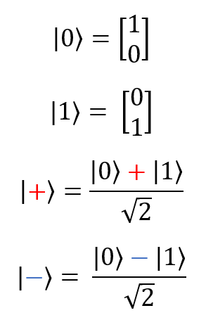 As these are all single-qubit pure states, we can represent them as points on the surface of the Bloch Sphere:
 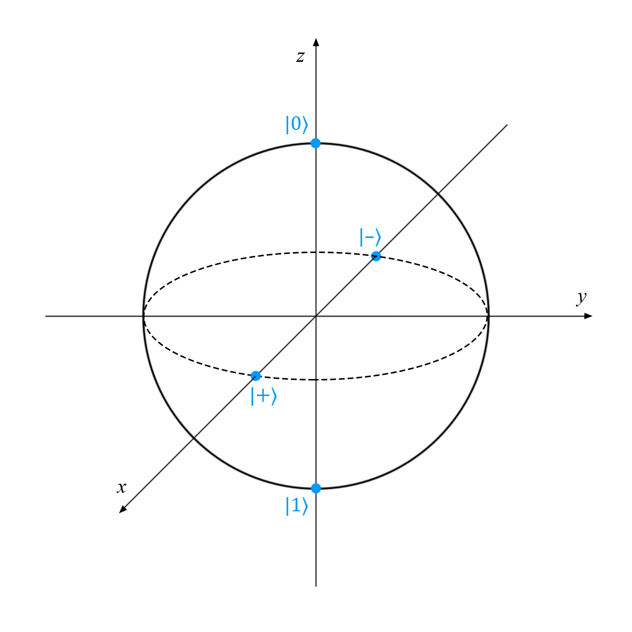 Now for the four Bell States, also known as EPR pairs after Einstein, Podolsky and Rosen who originally came up with the concept, later refined by John Bell. These are the simplest examples of quantum entanglement between two qubits:
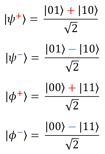
The last set of states we will introduce here are the GHZ (Greenberger-Horne-Zeilinger) states, shown below both in general form (for n qubits) and in its simplest (three-qubit) form: 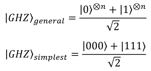
The Bell and GHZ states are important because they behave extremely non-classically due to the amount of entanglement present in the system – this concept of ‘maximal entanglement’ will be explored in a later post.
The Basics: Radians
When talking about quantum computing, rotations are measured in radians. Radians are simply a way of measuring angles in terms of π rather than in degrees – for example, there are 2π radians in a full circle. Angles are traditionally measured counter-clockwise. The diagram below shows the key conversions: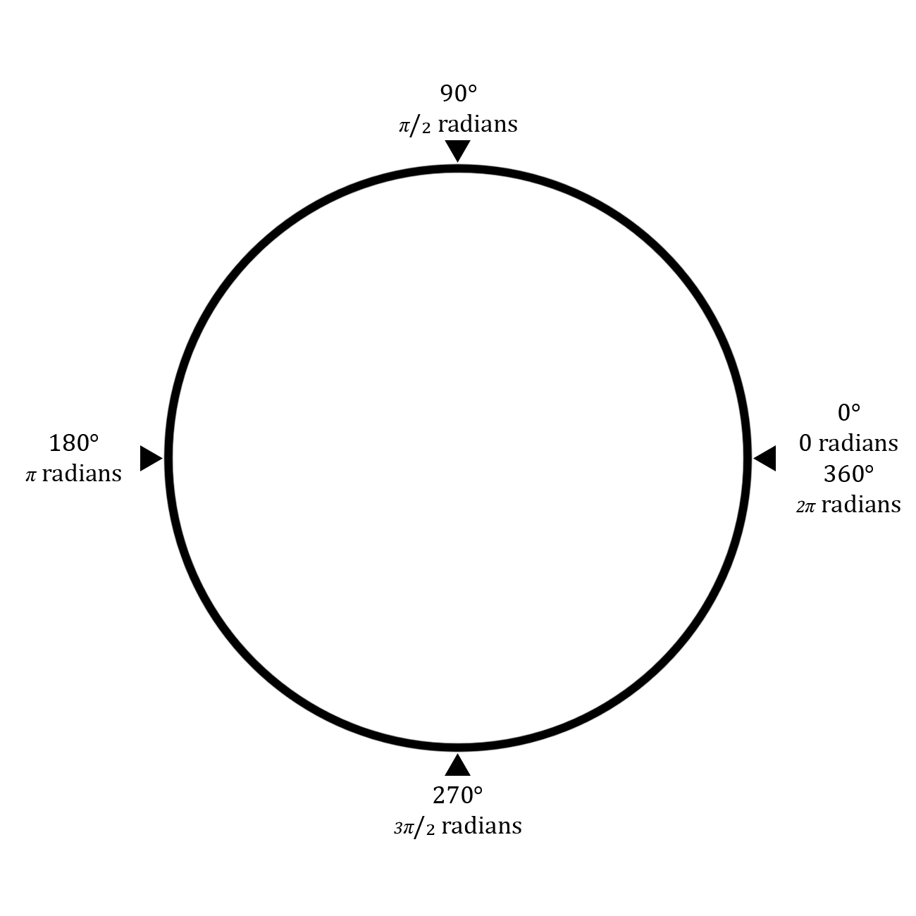
The Basics: Quantum Circuit Diagrams
Before we get stuck into learning about quantum gates, we first need to understand the basics of how quantum circuit diagrams are constructed (don’t worry, this won’t take long!):
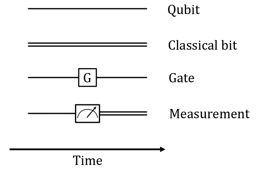
- In a circuit diagram, time moves from left to right
- Each qubit is represented by a single, horizontal line
- Most gates are represented by boxes, the letters/symbols within giving us information about what kind of gate it is
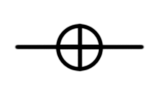
- The exceptions to this rule generally arise because there’s already a classical circuit element for the gate in question (e.g. the NOT gate)
- Some gates can have multiple diagram elements (e.g. NOT)
- The act of measuring a qubit causes any superpositions to collapse and its quantum properties to vanish, returning classical information. Hence, the measurement element below is seen to take in a qubit and output a classical bit. The Q# equivalent of this is
Measure(bases : Pauli[], qubits : Qubit[]), orM(qubit : Qubit)in the Z basis.
The key points are illustrated below:
Please refer to the documentation here, or alternatively Nielsen & Chuang’s Quantum Computation and Quantum Information for a more in-depth look at things.
Single-Qubit Gates
Single-qubit gates are (unsurprisingly) the simplest, so we will start there! You can visualise the operation of any single-qubit gate as the rotation of our qubit’s state to a different point on the Bloch Sphere (which I will illustrate here).
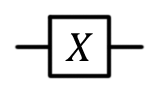
The three most basic single-qubit gates are the Pauli X, Y and Z gates:
| Name(s) | Matrix | Circuit Symbol(s) | Q# Representation |
|---|---|---|---|
| Pauli X, X, NOT, bit flip, |
 |
  |
X(qubit : Qubit) |
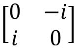
| Pauli Y, Y, |
 |
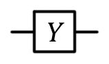 |
Y(qubit : Qubit) |
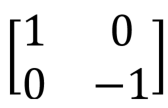
| Pauli Z, Z, phase flip, |
 |
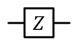 |
Z(qubit : Qubit) |
The X gate is directly analogous to the classical NOT gate – that is to say, it transforms |0〉 to |1〉 and |1〉 to |0〉. In terms of the Bloch Sphere, this is equivalent to rotating  around the x axis by π radians (180°).
Similarly, the Y gate represents a rotation of around the y axis by π radians. It transforms |0〉 to i|1〉 and |1〉 to -i|0〉.
The Z gate is actually a special case of the phase shift gate  (see below) where 𝜙 = π = 180°. It represents a rotation of around the z axis by π radians. It has no effect on |0〉 but transforms |1〉 to -|1〉.
Below we see these transformations mapped to the Bloch Sphere (the rotation axis in each case is highlighted red, click for larger image):![]()
It is important to note that applying the same Pauli gate to the same qubit twice in a row cancels out the operation (because you have now performed a full rotation of 2π (360°) over the surface to the Bloch Sphere, thus arriving back at the starting point). This brings us to the following fact: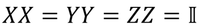 Because
  and so on, this is equivalent to:
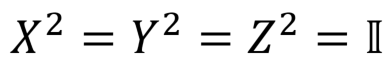 Where 𝕀 represents the identity matrix:
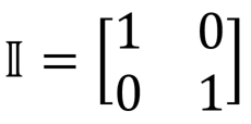 , which is the matrix equivalent of 1 (i.e. you can always multiply any matrix (M) by the identity (𝕀) to get the same matrix back again: M𝕀 = 𝕀M = M). Operationally the identity matrix can be thought of as an operation that does nothing to a quantum state. This can be seen on the Bloch Sphere:
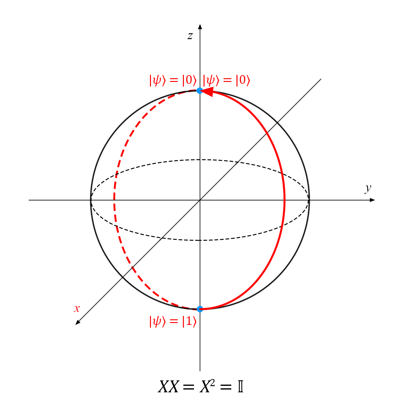
Because of this relationship, we say that the Pauli matrices are the square roots of the identity matrix.
Some other key single-qubit gates are detailed below:
| Name(s) | Matrix | Circuit Symbol(s) | Q# Representation |
|---|---|---|---|
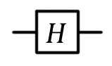
| Hadamard, H | 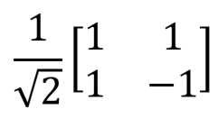 |
 |
H(qubit : Qubit) |
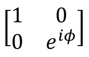
| Phase Shift, |
 |
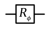 |
R1(theta : Double, qubit : Qubit) More generally: R(pauli : Pauli, theta : Double, qubit : Qubit) |
| Phase, |
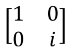 |
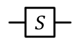 |
S(qubit : Qubit) |
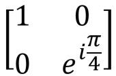 |
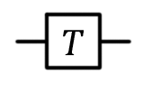 |
T(qubit : Qubit) |
The Hadamard gate is particularly important as it can be used to create a superposition of the |0〉 and |1〉 states. In the Bloch Sphere representation, it is easiest to think of this as a rotation of around the x-axis by π radians (180°) followed by a (clockwise) rotation around the y-axis by π/2 radians (90°):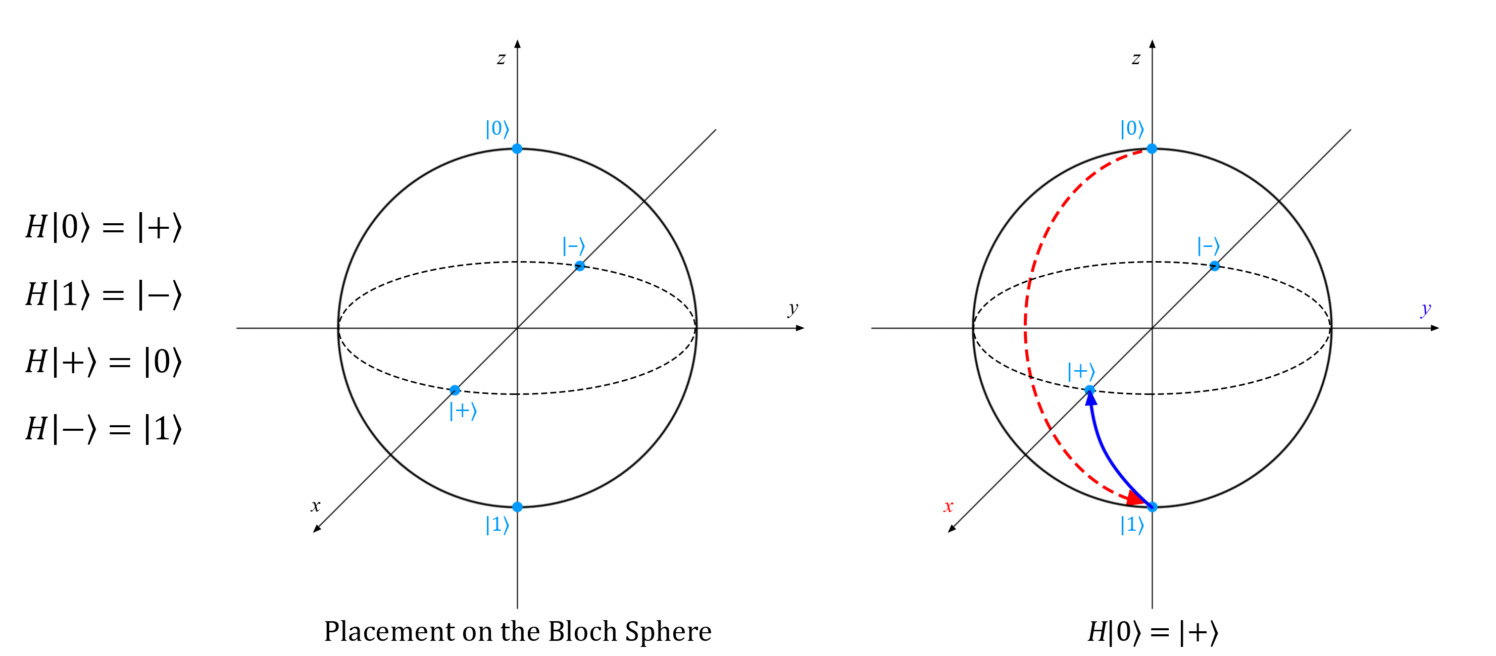
The phase shift gate is a generic gate that has many useful implementations, most notably the π/4, π/8 and Pauli-Z gates, which are generated by setting ϕ to π/2, π/4 and π, respectively. An example of a phase shift operation on is shown on the Bloch Sphere below: 
Multi-Qubit Gates
Multi-qubit gates work on two qubits or more. The SWAP gate is one of the simpler examples:
| Name(s) | Matrix | Circuit Symbol(s) | Q# Representation |
|---|---|---|---|
| SWAP | 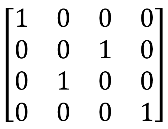 |
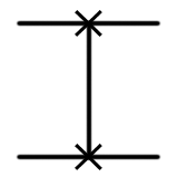 |
SWAP(qubit1 : Qubit, qubit2 : Qubit) |
The SWAP gate (unsurprisingly) swaps the two input qubits around. For example, SWAP|0〉|1〉 = |1〉|0〉 and SWAP|0〉|0〉 = |0〉|0〉 (see the circuits cheat sheet for the full truth table).
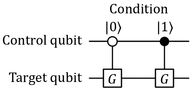
Another class of multi-qubit gates is the controlled gates. Controlled gates require at least one control and one target qubit – the gate in question will only operate on the target qubit if the control qubit is in a specific state.
If the gate requires the control qubit to be in the |1〉 state, this is denoted by a filled-in circle on the control qubit’s wire. If the condition is set on the control qubit being in the |0〉 state instead, we denote this with an empty circle, as seen below:
You can construct the matrix for any controlled gate by taking the identity matrix and attaching it to the top-left corner of the desired gate, then filling in the blank entries with zeroes, like so: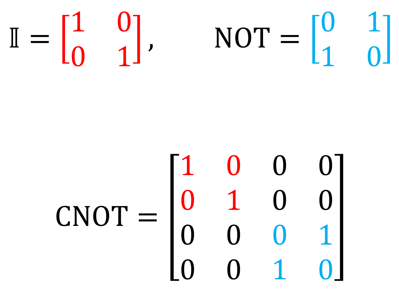
Controlled gates in Q# can be constructed from regular gates using the Controlled keyword as described here (under the ‘Controlled’ section at the very bottom of the page). For example, CNOT (remembering NOT is equivalent to the Pauli X gate) can be constructed as follows:
(Controlled X)([control], (target))
, where [control] represents an array of control qubits you feed in.
Some other common controlled gates are described below (I’ve highlighted the identity matrix in red and the original gate matrix in blue, as above):
| Name(s) | Matrix | Circuit Symbol(s) | Q# Representation |
|---|---|---|---|
| CNOT | 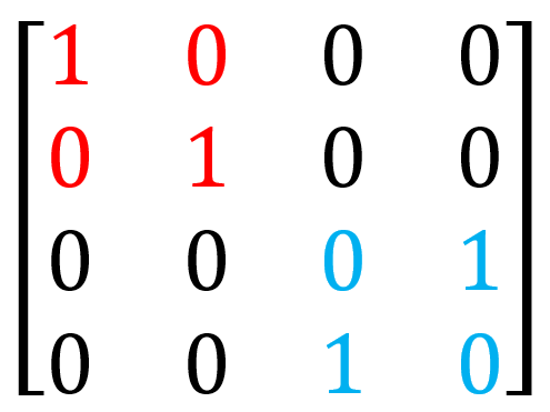 |
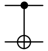 |
CNOT(control : Qubit, target : Qubit)or(Controlled X)([control], (target)); |
| CCNOT, Toffoli | 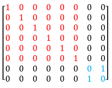 |
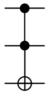 |
CCNOT(control1 : Qubit, control2 : Qubit, target : Qubit)or(Controlled X)([control1; control2], target); |
| CSWAP, Fredkin |  |
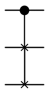 |
(Controlled SWAP)([control], (target)); |
Universal Sets
As mentioned in my first post, we must be able to implement a 'universal set' of gates for whichever physical system we are using as our quantum computer. This means that any computation possible on our system must decompose back into a finite sequence of known gates. For example, the Hadamard, phase, CNOT and π⁄8 gates together form one such universal set.
Universality is actually much more exciting than it looks at first. It means that any transformation permitted by quantum physics can be implemented on a quantum computer. This not only means we can run any quantum program; we can also use universality to run any physics. Universality therefore allows us to use a quantum computer to mimic molecules, super conductors and all manner of weird and wonderful quantum systems. In fact this ability of quantum computers to use universality simulate physics that can flummox even the best supercomputers promises to change the world. Not so boring right? 😊
More Excitement to Come!
Using these key gates (and some others), we can now start implementing full-blown quantum circuits! My next post will be all about how we can apply this new knowledge in the context of the Quantum Fourier Transform, a hugely important operation that has applications in all sorts of useful algorithms. See you there! 😃