Quantum Computing: Quick Reference Guide

Already understand the basics and just want to get stuck in? Can't quite remember what the CSWAP matrix looks like? This post is for you.

Here you will find a collection of all the main states/gates/matrices/useful maths bits/etc. covered so far in this blog series. This cheat-sheet will be updated as important new things are introduced in posts 😊 

For all posts past and future, please refer to the Hitchhiker's Guide to the Quantum Computing and Q# Blog.

• The Bloch Sphere
• Key Quantum States
• Gates, Matrices and Operations
• Useful Relationships and Equations

Any unitary transformation we do on |𝜓〉 can be visualised as simply moving the point (marked |𝜓〉) around the Bloch Sphere*. Sadly, this visualisation can only be used for single qubit states, as there is no known (simple) generalisation that applies to multi-qubit systems. You may also see it referred to in places as the Unit Sphere.

*All pure states can be found on the surface of the sphere, whereas mixed states are located within the sphere. Please refer to my other post Quantum Computing Primer: Pure vs. Mixed States for further explanation.

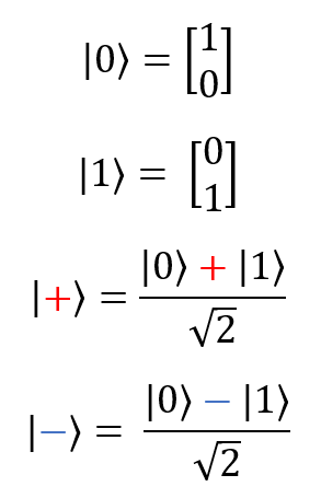
Single-qubit states:

Bell States/EPR pairs - these are the simplest examples of quantum entanglement between two qubits:

GHZ (Greenberger-Horne-Zeilinger) states, shown below both in general form (for n qubits) and in its simplest (three-qubit) form:

Below is a summary of the key gates as introduced in my previous post about Gates and Circuits. Operations have been included for all single- and two-qubit gates (three plus becomes too big for display). For controlled gates, the identity matrix (𝕀) has been higlighted red and the original gate matrix blue, as seen previously.

Name(s)	Matrix	Circuit Symbol(s)	Q# Representation	Key Operations
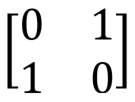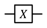Pauli X, X, NOT, bit flip,			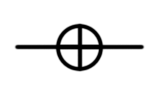X(qubit : Qubit)
Pauli Y, Y,			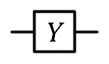Y(qubit : Qubit)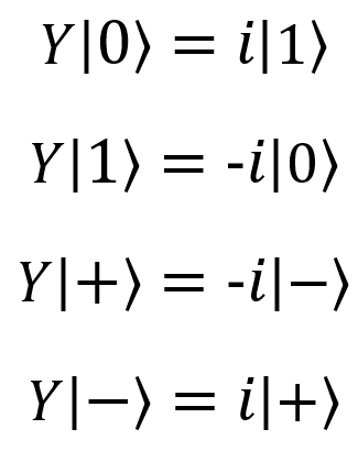
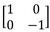
Pauli Z, Z, phase flip,			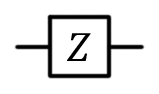Z(qubit : Qubit)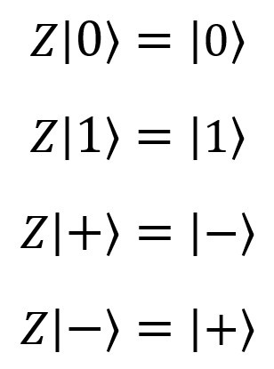
Hadamard, H		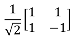	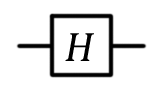H(qubit : Qubit)
Phase Shift,			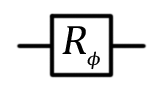R1(theta : Double, qubit : Qubit) More generally: R(pauli : Pauli, theta : Double, qubit : Qubit)
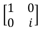
Phase,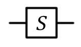, S			S(qubit : Qubit)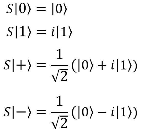
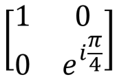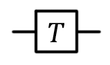, T			T(qubit : Qubit)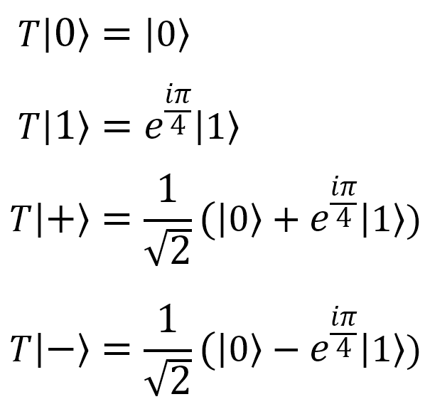
SWAP			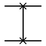SWAP(qubit1 : Qubit, qubit2 : Qubit)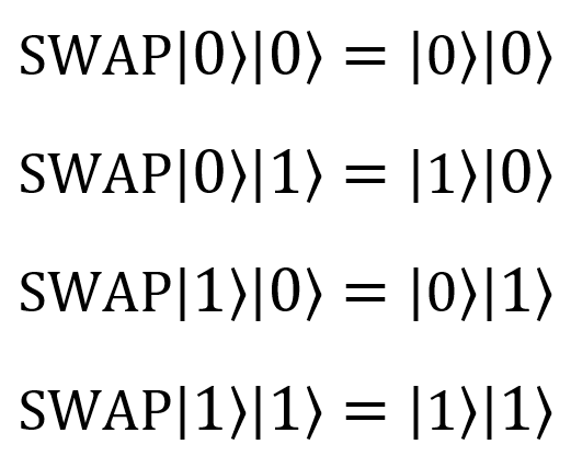
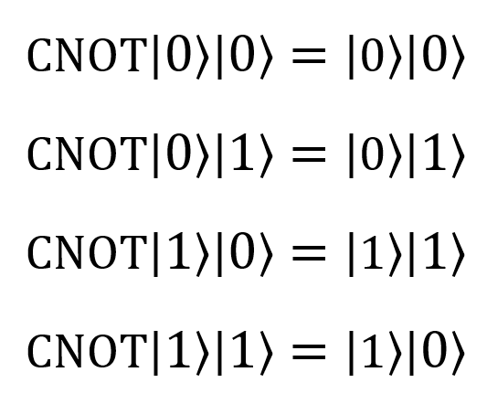
CNOT		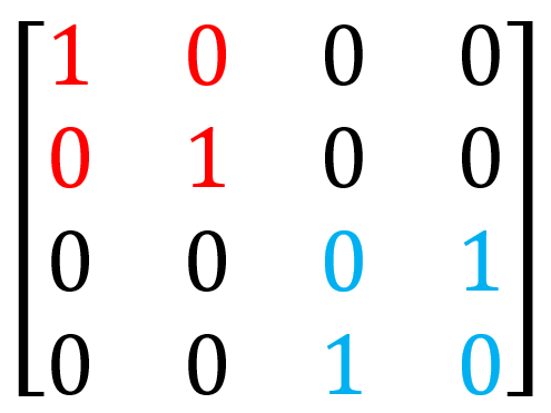	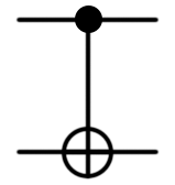CNOT(control : Qubit, target : Qubit)or(Controlled X)([control], (target));
CCNOT, Toffoli		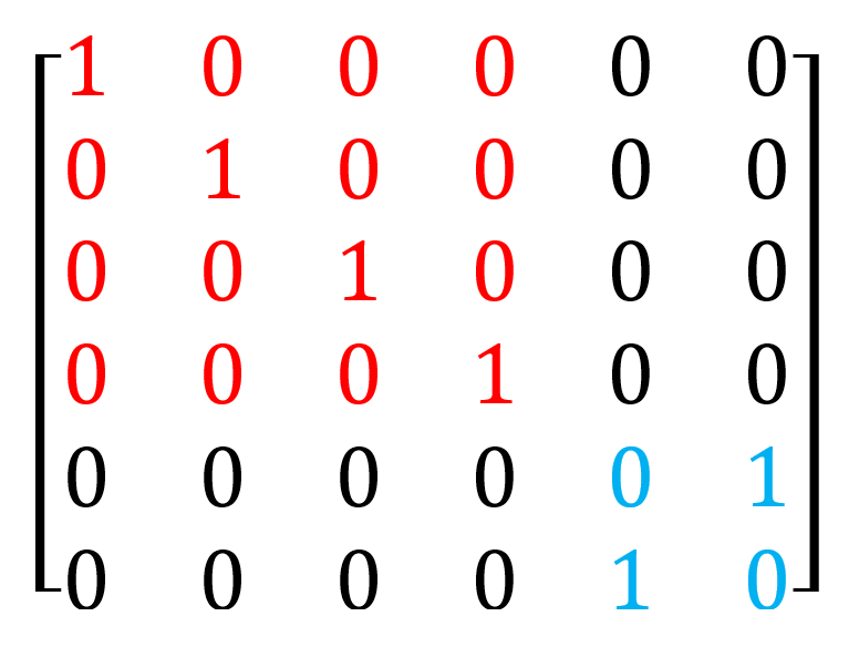	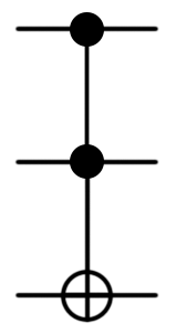CCNOT(control1 : Qubit, control2 : Qubit, target : Qubit)or(Controlled X)([control1; control2], target);	-
CSWAP, Fredkin		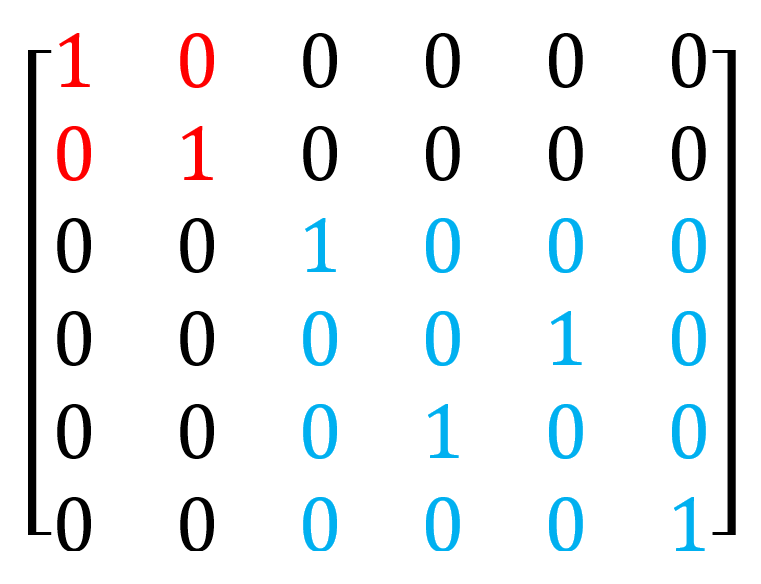	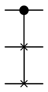(Controlled SWAP)([control], (target));	-

The Pauli matrices are their own inverse:

The density operator can be defined as follows:

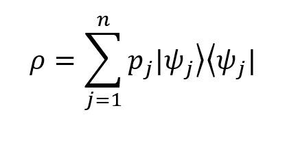
Where:

• is the probability of the system being in state at the start.
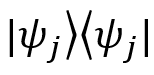• The element represents the outer product of the vector with itself, which produces a matrix (this is also known as a projection operator).
• n is the total number of possible states the system could be in (in our example, 3).
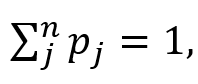• as you would expect (the sum of the probabilities for all possible states is equal to 1)

 Learn more at the Microsoft Quantum website: https://www.microsoft.com/en-us/quantum/

Download the Quantum Development Kit: https://www.microsoft.com/en-us/quantum/development-kit

Stay up to date with the Microsoft Quantum newsletter: https://info.microsoft.com/Quantum-Computing-Newsletter-Signup.html

Read about the latest developments on the Microsoft Quantum blog: https://cloudblogs.microsoft.com/quantum/

Twitter: https://twitter.com/MSFTQuantum

Facebook: https://www.facebook.com/MicrosoftQuantum/

• Anonymous
  March 16, 2018
  Hey Anita & Frances!Big Thanks for this great and approachable Intro into Quantum!Can't await to finally understand QFT!!!!Keep up the excellent work!/*Karl