Getting started with R · Arithmetic and logical operators, Objects, Vectors, Factors & Lists
Guest post by Slaviana Pavlovich Microsoft Student Partner
I am an IT and Management student at University College London with a passion for data science. I recently completed the Microsoft Professional Program for Data Science, where I developed core skills to work with data. If you are also interested in this career, but not sure where to start - I strongly encourage you to check it out. I also have a wide range of interests including 3D bioprinting, public speaking, and politics. Additionally, I enjoy swimming and photography to balance out my studies. I became a Microsoft Student Partner at the end of my first year and I absolutely enjoy being part of such a vibrant community. If you have any questions, feel free to ask!
Introduction
In today’s article, I am going to talk about R programming language that was originally developed by and for statisticians and then became widely accepted by data scientists as well. In the first part of this two-part introduction to R, we are going to consider:
· What is R and how to install RStudio
· Arithmetic and logical operators
· Objects
· Vectors
· Factors
· Lists
What is R and how to install RStudio
In 2006, Clive Humby (UK mathematician and architect of Tesco’s Clubcard) said: “Data is the new oil. It’s valuable, but if unrefined it cannot really be used. It has to be changed into gas, plastic, chemicals, etc. to create a valuable entity that drives profitable activity; so must data be broken down, analyzed for it to have value.”
R is going to be our tool for getting the value out of data. As said on the official website, R is an open-source programming language and software environment for statistical computing and graphics (1). There are certain benefits of using R language:
· One of the main benefits of R and RStudio that they are both free and user-friendly. R is not just for advanced programmers, so everyone can have a go!
· Another benefit of R is its stability and reliability because, as mentioned above, it goes under an open-source license. It means that talented programmers contributed to the R code to make it excellent.
· It should also be mentioned that R compiles and runs on a variety of platforms, including Windows, Linux and MacOS.
· R is a powerful language with thousands of packages. There are multiple packages for data manipulation and plotting, for example the ggvis and ggplot2 are very popular packages for this.
· Finally, there is an amazing engaged community of R enthusiasts.
After reading about R, you might already have a burning desire to start, so let’s not wait!
1) Install R.
· Follow the link and then choose the operational system you use. In my case, it is Windows.
· Choose the option ‘install R for the first time’ and download the setup file.
· Open the downloaded file and Install R.
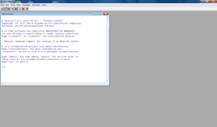
· Run the installation file and you will be able to see the standard version of the console.
2) Install RStudio.
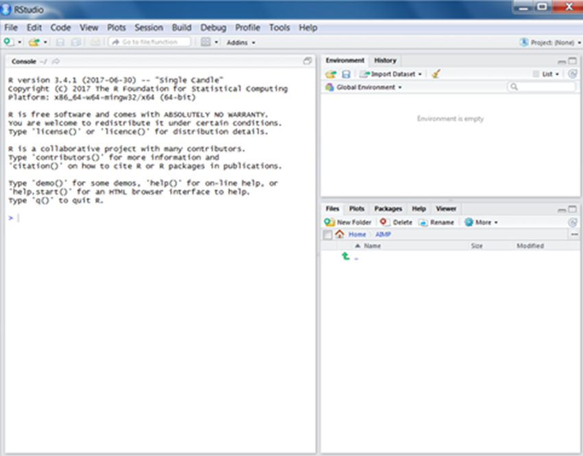
RStudio is an integrated development environment for R, in simple terms, a code editor.
· Follow the link and click the Download RStudio Desktop button.
· Open the downloaded .exe file and Install RStudio.
· After RStudio is installed, find and launch it.
Arithmetic and logical operators
Time to execute your first command! As most of the programming languages, R can perform basic arithmetic operators. For example, enter ‘68+2’ at the prompt and you will see the following:
 > 68+2
 [1] 70
! Remember, each command is executed one at a time in R.
There is a certain number of operations that R can do, such as addition (+), substraction (-), multiplication (*), exponentiation (^ or **), division (/) and modulo (%%).
 > 68-2
 [1] 66
 > 68*2
 [1] 136
 > 3^4
 [1] 81
 > 3**4
 [1] 81
 > 25/5
 [1] 5
 > 25%%5
 [1] 0
As they say, practice makes perfect. That is why I encourage you to try these operations on your own right now.
! Remember, if you want to leave a comment use a hash ( # ); leaving comments is crucial, because it will help you or someone else to understand your code better. Also, comments are ignored by the compiler. In fact, they are treated as whitespace.
 > #Let's leave a comment!
 > 3+3 #Another comment
 [1] 6
As a test, in the example above, at first I left only the comment and then after I put an arithmetic operation and then the comment. In both examples the comments are ignored.
After considering arithmetic operators, I suggest looking at logical operators that are there: exact equality (==), exact inequality (!=), less than (<), less than or equal to (<=), greater than (>), greater than or equal to (>=):
 > 68 != 68
 [1] FALSE
 > 68 == 68
 [1] TRUE
 > 1 <= 2
 [1] TRUE
 > 7 >= 4
 [1] TRUE
 > 8 < 3
 [1] FALSE
In ordinary arithmetic, these logical operators have the value either TRUE (1) or FALSE (0), as shown above.
Objects
To create new variables, you will need to use the assignment operator ( <- ):
 > # Creating a new variable 'article' that has the value of 2
 > article <- 2
 > # Printing it out
 > article
 [1] 2
 > article + 7
 [1] 9
Instead of declaring data types, as done in C++ and Java, in R, the user assigns the variables with certain Objects in R, the most popular are:
· Vectors
· Factors
· Lists
· Data Frames
· Matrices
The data type of the object in R becomes the data type of the variable by definition.
Vectors
There are six data types of the simplest object - vector:
· Logical
· Numeric
· Integer
· Character
· Raw
· Complex
! Remember, if you want to check the variable type, use class() .
 > a <- FALSE
 > class(a)
 [1] "logical"
 > b <- 45.77
 > class(b)
 [1] "numeric"
 > c <- 7
 > class(c)
 [1] "numeric"
 > d <- 8L # L is used to indicate that it is a natural number
 > class(d)
 [1] "integer"
 > e <- 71 + 2i
 > class(e)
 [1] "complex"
To create the vector that has more than one element, you will need to use the function c() that combines the elements into a vector:
 > # Creating a vector
 > object <- c(1, 19, 7 + 1, 123)
 > object
 [1]   1  19   8 123
 > class(object)
 [1] "numeric"
As we can see above, the class of this vector is numeric, since all the elements of the vector are of the same data type.
 > example <- c("Penguin", "Squirrel")
 > example
 [1] "Penguin"  "Squirrel"
 > class(example)
 [1] "character"
Vectors can contain different elements, but will store them as one type.
For example, assume that there are logical, numeric and character elements, automatic coercion (logical<numeric<character) takes place, since vectors are homogeneous:
 > V <- c(TRUE, "penguin", 77)
 > V
 [1] "TRUE"    "penguin" "77"
 > class(V)
 [1] "character"
You can also perform arithmetic operations on vectors:
 > a <- c(7,15,20)
 > b <- c(10,14,21)
 > a + b
 [1] 17 29 41
 > a - b
 [1] -3  1 -1
 > a * b
 [1]  70 210 420
 > a / b
 [1] 0.700000 1.071429 0.952381
 > a^2 + b
 [1]  59 239 421
 > a - 1
 [1]  6 14 19
All the operations are done element-wise, as you can see above.
! Remember, to list all current objects use a function ls() and rm() to remove.
To select a specific element of a vector, you will need to use the subset function “ [] ”:
 > # Creating a vector
 > v <- c(77, 1, 31, 4)
 > v[2] # Selecting element that has index 2
 [1] 1
 > v[c(1,3)] # Selecting elements at index 1 and 3
 [1] 77 31
 > v[2:4] # Selecting a subset of elements from 2nd to 4th
 [1]  1 31  4
Factors
Factors are objects in R that are created using a vector. It is very common to use factors in statistical modelling. Factors store the vector, as well as the set of values that are used when the factor is printed. To create a factor, you will need to use a function factor() . Let’s look at the following example:
 > # Creating a vector
 > shoe_sizes <- c(38, 40, 36, 42, 36, 40, 41)
 > # Creating a factor object
 > factor_sizes <- factor(shoe_sizes)
 > # Print out the factor
 > factor_sizes
 [1] 38 40 36 42 36 40 41
 Levels: 36 38 40 41 42
 > # Show the number of levels
 > nlevels(factor_sizes)
 [1] 5
Numeric and character variables can be used to create a factor, but levels of factors are always going to be character variables. The levels of a factor are used when the factor is printed. If you want to change the way the levels are displayed, use labels. This will also change the internal levels of a factor:
 > clothes_sizes <- c("Small", "Medium", "Large", "Small", "Large", "Small", "Large")
 > factor_clothes <- factor(clothes_sizes, labels = c("L", "M", "S"))
 > factor_clothes
 [1] S M L S L S L
 Levels: L M S
Lists
We learned before that vectors are homogeneous. Unlike vectors, lists are heterogeneous. Lists can consist of different objects, such as vectors, arrays etc. It is also possible to have a list inside of the list. Let’s look at the examples below:
 > # Creating a list that contains 4 elements
 > example <- list(71, c(10,18,19), "R is great!", TRUE)
 > example
 [[1]]
 [1] 71

 [[2]]
 [1] 10 18 19

 [[3]]
 [1] "R is great!"

 [[4]]
 [1] TRUE

 > # Creating a list that has 2 lists
 > twolists <- list("R is fun!", example)
 > twolists
 [[1]]
 [1] "R is fun!"

 [[2]]
 [[2]][[1]]
 [1] 71

 [[2]][[2]]
 [1] 10 18 19

 [[2]][[3]]
 [1] "R is great!"

 [[2]][[4]]
 [1] TRUE
Resources
https://academy.microsoft.com/en-us/professional-program/ Microsoft professional programmes, Big Data, Data Science
https://imagine.microsoft.com/en-us/Catalog R Server Download for Students & Academics via Imagine Access
https://docs.microsoft.com/en-us/r-server/ R Server and R Documentation
https://www.microsoft.com/en-gb/cloud-platform/r-server Microsoft R Server
https://docs.microsoft.com/en-us/visualstudio/rtvs/ R for Visual Studio Docs
https://www.visualstudio.com/vs/rtvs/ R for Visual Studio
https://www.rstudio.com/ R Studio


