Measuring spam effectiveness – the flip side of false positives
As I was saying in my previous post, when it comes to measuring effectiveness you need to take a lot of samples in order to do it properly from a statistical point of view. This makes it difficult to attain accurate metrics unless you have a pretty impressive infrastructure.
The flip side, measuring how well you do against spam, is actually quite a bit easier. The reason is that it is relatively easy to attain feeds of spam in high volumes. Spam makes up 90% of email traffic on the Internet (excludes private intra-org mail) and it changes all the time, every day in fact. And so setting up a few hundred honeypots will take a bit of time to get them up and going but once you do it will be smooth sailing. To be sure, every few months or so you will need to retire those honeypots and also ensure that gray mail doesn’t somehow get into them, but at least you can be certain that spammers will never stop sending to it and you don’t need their consent to siphon off that mail since it is mail destined to a domain that you own. The only problem is ensuring that the spam you get is representative of a large enough swath of the spam ecosphere.
To look at the nuances of spam filtering and comparing them side-by-side, suppose you have three products. For the sake of argument we will call them A, B and C. You take a certain number of messages, run them through and on the first day of your test you get the following results:
Filter A – 97.7%
Filter B – 98.2%
Filter C – 92.4%
Filter B has the highest effectiveness and therefore it is the best filter. Case closed, right? The answer is not quite yet.
When doing measurements, you invariably have to do statistical sampling. This is because the only way you can measure something definitively (in anything) is to measure the entire population. In our case, to do a real test you’d have to measure the 1 trillion spam messages that are sent each day and nobody can get access to all of the world’s spam. Fortunately, you don’t have to do that.
In public opinion polls, or election polls, polling organizations often publish results showing Candidate X is ahead of Candidate Y. This is well-understood technology (by statisticians, not necessarily by the general public). As long as you take a large enough sample size and do a random sample, the results of your sample will be more or less representative compared to what the results would be if you polled the entire population. In other words, if you randomly sampled 1000 people and 60% said that they would vote for Candidate X and 40% said that they would vote for Candidate Y, then on election day Candidate X would get approximately 60% of the vote while Candidate Y would get approximately 40% of the vote.
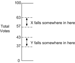
Note that I say approximately. This is because in statistical sampling, you are only doing a random sample of the population and therefore there is always going to be room for error. If you were to take the test over again, then the numbers might not be 60/40. Instead, they could be 61/39, or 59/41. The amount of error is dependent on the size of the sample. This is calculated using mathematical formulae, but the larger the sample size, the smaller the margin of error. So, given that, let’s return to our example above. Candidate X would get 60% of the vote and Candidate Y would get 40% of the vote. In actuality, X would get 60% ±3.1%, and Y would get 40% ± 3.1% (3.1% is the margin of error you can calculate statistically).
Viewing it this way, then based upon 1000 people who say who they would vote for, then the worst-case scenario for X is 57% and the best case scenario for Y is 43%. There is no way that Y can be better than X and therefore you can truly say that X is ahead in the race against Y. One thing to note is that in statistics, we have the concept of a confidence interval. If you use the 95% confidence interval, then based upon a sample of 1000 people, then we are 95% sure that X’s true percentage is between 57 and 63. Or, to put it another way, if we did the test 20 times, 19 of those times would have X’s percentage between 63 and 57.
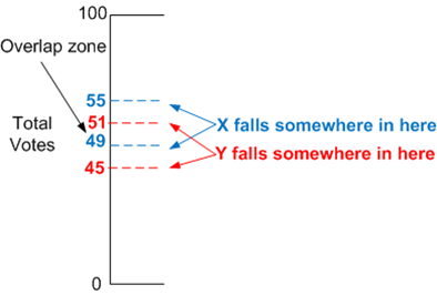
What happens if you do a poll and X gets 52% and Y gets 48%? Is X winning? The answer from a statistical point of view is: Inconclusive. This is because at 1000 samples, the margin of error is overlapping. I will color-code X in blue and Y in red:
You can see from the diagram above that there is an overlap zone between 51% and 49%. If you did the test over again there is a chance that X could get 49.5% and Y could get 50.5% (this could also be the actual result on election day). This means that the winner between the two candidates would be the opposite of what was predicted on polling day if all you looked at was the original 52/48 split. However, statistically speaking, the reversal of fortune on election day was a possible scenario that was allowed for by the polling data because the margin of error permitted that much movement.
So how do you get rid of this overlap zone? Simple. Increase the number of samples such that the margins of error do not overlap. If you did the test over again and got the same 52/48 split, but this time sampled 5000 participants instead of 1000, the margin of error is 1.38% (at the 95% confidence interval). This means that Candidate X has 52% ± 1.38% and Candidate Y has 48% ± 1.38%. The minimum number of votes that X has is 50.62% and the maximum that Y has is 49.38%. That’s a margin of difference of 1% of non-overlap; it’s close, but X is definitely leading Y by a small amount and would win the election if it were held today.
Returning back to our spam filtering problem, remember our results:
Filter A – 97.7%
Filter B – 98.2%
Filter C – 92.4%
No test runs all of the world’s spam through the competing vendors, it’s all done using a down sample of it. We have three questions to ask ourselves:
Was the spam randomly sampled? If you are an organization that gets one type of spam, then you can tune your filter for it. However, to be fair, you should cut a wide enough swath to ensure that you are getting a representation of all of the spam on the Internet, not just one narrow band. Now, your sample might be heavier weighted in one kind vs another (pharmaceutical spam vs 419s) but if you do it right, having more of one category of spam in your sample is perfectly fine because that’s what the entire spam population looks like. Acquisition of a suitable corpus, however, is out-of-scope of this blog post.
Is the sample size large enough? In our example, Filter A is below filter B by 0.5%. However, remember our margins of error. These numbers only matter if the margins of error are large enough to ensure that there is no overlap area and therefore the margins don’t matter. For something this close (0.5% difference), you need 164,002 samples. This gives filter A an effectiveness of 97.7% ± 0.24% (max 97.94%) and filter B an effectiveness of 98.2% ± 0.24% (min 97.96%). Those are very close, but Filter B is juuuuuuust a little bit better than Filter A.
What is the timing of the test? Was it done over one day or several days? Any one filter can have a good day and a bad day. To be fair and average things out over a longer period of time, a test should be performed over a longer time period (a couple of weeks) and then the results averaged out.
So there you have it. The bottom line is that when it comes to spam filtering, you need a lot of samples and you need to do it over a period of time. Without those two, your results might look good but no conclusions can be drawn.

