Math Primer Series: Matrices III: Affine Transformations and Matrices

We’ve seen matrices used as representations of a basis, and we’ve seen them used as linear transformations, but what else can we do with them? So far, we’ve only been able to use matrices to transform vectors from one vector space to another. What about points and vectors in an affine space? There is another class of transformation, called an affine transformation, which does exactly this.

Affine Transformations

An affine transform is a transformation which maps points and vectors in an affine space to another affine space. This allows us to transform positions now, in addition to just vectors. An affine transformation can be thought of as a combination of a basis matrix and a translation to an origin, which is analogous to affine spaces compared to vector spaces, since affine spaces add an origin. When we look at an object, we can define a right, up, and forward vector for it, relative to some frame of reference. But furthermore, we can describe it’s position in space. Not the position of a particular point on the object, but the position of the whole object. What we’re actually doing is saying that all the points on the object can be thought of relative to some origin on the object, and that origin has a location in space (relative to some frame of reference of course). This means that even though we move the object’s origin around, we’re not changing the orientation (the right, up, and forward vectors). The reverse is also true, we can rotate or scale our object all we want, but it won’t move the object’s origin. In this way, we see that the origin of the object, and it’s basis are independent, and the formal affine definition reflects this separation. Affine transformations are formally defined as multiplying a point by a matrix component (to define it’s orientation) and then adding a vector component (to define it’s origin’s position):

Here, M is the matrix portion of the transformation, and is sometimes referred to as the linear portion. This can consist of rotation, scaling, or any other linear transformation. The t in the equation is called the translation and is the vector defining where the object’s origin is compared to some frame of reference. Let’s take a look at an example to get a better grasp of this:

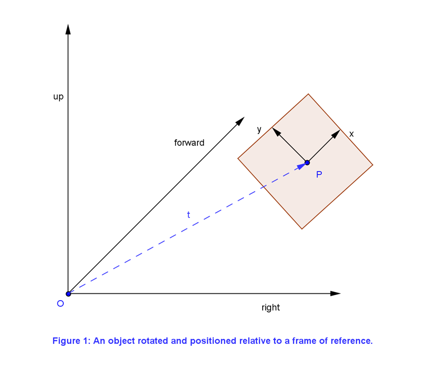
In Figure 1, we see a frame of reference shown (origin O, with right, up, and forward defining our frame). We also see an object (the square). If we were locally sitting inside that object, then x and y would have been our right and up vectors, and P our local origin. But since we’re examining the object from a different frame of reference, it appears rotated and located at some other location. This placement and orientation can be described as a single affine transformation, as show in the equation above, with M being the linear portion and t being the translation portion. Using our example above, and assuming only rotation (to simplify), our matrix M would likely look like:

Assuming that x, y, and z (which we can’t see in the image) are defined relative to our coordinate space and are unit length. Look back to this post if you’re unsure how we got that. We then would add our translation vector (dashed line t in the figure).

While this works out well enough, the extra addition must be remembered and there’s not a convenient way to store this information. Fortunately, there’s an alternate way to express and use affine transformations which is much more convenient and consistent with what we’ve already seen:

Note that this is now a 4x4 matrix, as apposed to the usual 3x3 we’ve seen so far. It contains the linear part of the affine transformation in the upper left 3x3 block, and the translation vector as the last column. The bottom row contains 0s with the exception of the last entry which is a 1. Here’s an example of the expanded matrix from the previous example:

Before we go on, I wanted to call out that I’ve been using column matrices so far in this post. The same concepts apply if you’re using row matrices, just remember the layout will be transposed from what I’m showing here, with the translation vector as the bottom row of the matrix, and the 0s as the last column, and transposing the upper left block.

Now, we claimed earlier that affine transformations could be used to transform both points and vectors from an affine space to another. Points and vectors are quite different. One is a location and one is a direction. It doesn’t make any sense to translate a direction, so how can we possibly use this matrix to transform vectors? The answer is in the fact that we have to augment a point or vector to be compatible with this matrix. This is a 4x4, and both points and vectors are 3 components. Without some augmentation, the points and vectors are not compatible with this new matrix. How we augment them depends on whether they are points or vectors, and dictates whether the translation component of the affine matrix is applied or not.

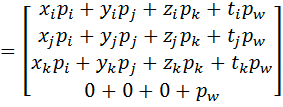
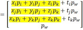
If you recall from this post, points are sometimes written as 4 component vectors with a 1 in the last component (sometimes called w). Vectors can likewise be written with 4 components, with the last component equal to 0. The reasons this worked for arithmetic were shown in the post, but we now see there is another critical reason for that distinction. When you multiply a 4 element vector with the affine matrix above, the math works out to:

Note the highlighted portion of the last one there. This is exactly what you’d get using a normal 3x3 transform M multiplied by p. This means that we get the exact same result as applying the linear transformation M and then adding t times p’s w component. If the w component is 0, as in the vector case, it cancels out the translation portion. If the w component is 1, then we translate by exactly t, which is what we expect for points. Notice also that the last element of the new vector is exactly equal to the w component of the starting vector. This means that vectors stay vectors under affine transformation, and points stay points. This is pretty important, it means that an affine space will never turn points into vectors or vice versa. The augmented points and vectors which contain the w component are said to be in homogenous space, and another term often used for the affine matrix (since it requires homogenous vectors) is a homogenous matrix.

In the next and final matrix-related math primer post, we’ll examine some other operations which can be performed on matrices. Specifically, we’ll take a look at the determinant, adjunct, and inverse. Afterwards, we’ll quickly look at some of the problems with rotations, and introduce quaternions as an alternative way to express rotations which overcomes many of the traditional problems. I’m going to be continuing the physics posts as well.