How to Read Statistics Profile
(2006-09-01 added a paragraph on parallel query plans)
In SQL Server, “Statistics Profile” is a mode in which a query is run where you can see the number of invocations of each physical plan operator in the tree. Instead of running a query and just printing the output rows, this mode also collects and returns per-operator row counts. Statistics Profile is used by the SQL Query Optimizer Team to identify issues with a plan which can cause the plan to perform poorly. For example, it can help identify a poor index choice or poor join order in a plan. Oftentimes, it can help identify the needed solution, such as updating statistics (as in the histograms and other statistical information used during plan generation) or perhaps adding a plan hint. This document describes how to read the statistics profile information from a query plan so that you can also debug plan issues.
A simple example query demonstrates how to retrieve the statistics profile output from a query:
use nwind
set statistics profile on
select * from customers c inner join orders o on c.customerid = o.customerid;
The profile output has a number of columns and is a bit tricky to print in a regular document. The key pieces of information that it prints are the plan, which looks like this:
StmtText
------------------------------------------------------------------------------------------------------
select * from customers c inner join orders o on c.customerid = o.customerid
|--Hash Match(Inner Join, HASH:([c].[CustomerID])=([o].[CustomerID]),
|--Clustered Index Scan(OBJECT:([nwind].[dbo].[Customers].[aaaaa_PrimaryKey] AS [c]))
|--Clustered Index Scan(OBJECT:([nwind].[dbo].[Orders].[aaaaa_PrimaryKey] AS [o]))
Other pieces of useful information are the estimated row count and the actual row count for each operator and the estimated and actual number of invocations of this operator. Note that the actual rows and # of executions are physically listed as early columns, while the other columns are listed later in the output column list (so you typically have to scroll over to see them).
Rows Executes
-------------------- --------------------
1078 1
1078 1
91 1
1078 1
EstimateRows
------------------------
1051.5834
1051.5834
91.0
1078.0
EstimateExecutions
------------------------
NULL
1.0
1.0
1.0
Other fields, such as the estimated cost of the subtree, the output columns, the average row size, also exist in the output (but are omitted for space in this document).
Note: The output from statistics profile is typically easiest to read if you set the output from your client (Query Analyzer or SQL Server Management Studio) to output to text, using a fixed-width font. You can then see the columns pretty easily and you can even move the results into a tool like Excel if you want to cluster the estimates and actual results near each other by rearranging the columns (SSMS also can let you do this).
There are a few key pieces of information needed to understand the output from Statistics profile. First, query plans are generally represented as trees. In the output, children are printed below their parents and are indented:
StmtText
------------------------------------------------------------------------------------------------------
select * from customers c inner join orders o on c.customerid = o.customerid
|--Hash Match(Inner Join, HASH:([c].[CustomerID])=([o].[CustomerID]),
|--Clustered Index Scan(OBJECT:([nwind].[dbo].[Customers].[aaaaa_PrimaryKey] AS [c]))
|--Clustered Index Scan(OBJECT:([nwind].[dbo].[Orders].[aaaaa_PrimaryKey] AS [o]))
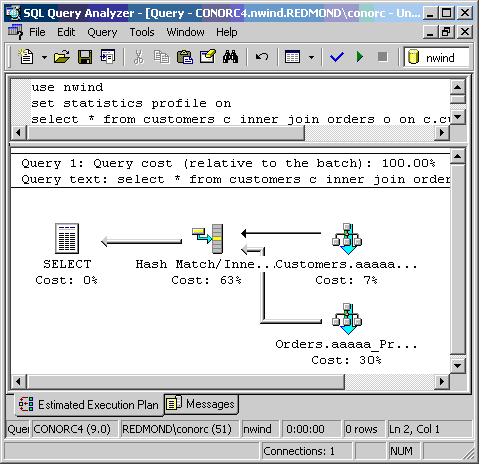
In this example, the scan of Customers and Orders are both below a hash join operator. Next, the “first” child of the operator is listed first. So, the Customers Scan is the first child of the hash join. Subsequent operators follow, in order. Finally, query execution plans are executed in this “first” to “last” order. So, for this plan, the very first row is returned from the Customers table. (A more detailed discussion of operators will happen later in the article). Notice that the output from the graphical showplan is similar but slightly different:
(see attachment tree.jpg).
In this tree representation, both Scans are printed to the right on the screen, and the first child is above the other operators. In most Computer Science classes, trees are printed in a manner transposed from this:
Hash Join
/ \
Customers Orders
The transposition makes printing trees in text easier. In this classical view, the tree is evaluated left to right with rows flowing bottom to top.
With an understanding of the nuances of the query plan display, it is possible to understand what happens during the execution of this query plan. The query returns 1078 rows. Not coincidentally, there are also 1078 orders in this database. Since there’s a Foreign Key relationship between Orders and Customers, it requires that a match exist for each order to each customer. So, the 91 rows in Customers match the 1078 rows in Orders to return the result.
The query estimates that the join will return 1051.5834 rows. First, this is a bit less than the actual (1078) but is not a substantial difference. Given that the Query Optimizer is making educated guesses based on sampled statistical information that may itself be out-of-date, this estimate is actually pretty good. Second, the number is not an integer because we use floating point for our estimates to improve accuracy on estimates we make. For this query, the number of executions is 1 for both the estimate and actual. This won’t always be the case, but it happens to be true for this query because of the way hash joins work. In a hash join, the first child is scanned and a hash table is built. Once the hash join is built, the second child is then scanned and each row probes the hash table to see if there is a matching row.
Loops join does not work this way, as we’ll see in a slightly modified example.
select * from customers c with (index=1) inner loop join orders o with (index=1) on c.customerid = o.customerid
In this example, I’ve forced a loop join and the use of clustered indexes for each table. The plan now looks like this:
StmtText
-----------------------------------------------------------------
select * from customers c with (index=1) inner loop join orders o
|--Nested Loops(Inner Join, WHERE:([nwind].[dbo].[Orders].[Cust
|--Clustered Index Scan(OBJECT:([nwind].[dbo].[Customers].
|--Table Spool
|--Clustered Index Scan(OBJECT:([nwind].[dbo].[Orders
Beyond the different join algorithm, you’ll notice that there is now a table spool added to the plan. The spool is on the second child (also called the “inner” child for loops join because it is usually invoked multiple times). The spool scans rows from its child and can store them for future invocations of the inner child. The actual row count and execution count from the statistics profile is a bit different from the previous plan:
Rows Executes
-------------------- --------------------
1078 1
1078 1 <--- Loop Join
91 1 <--- Scan of Customers
98098 91 <--- Spool
1078 1 <--- Scan of Orders
In this plan, the second child of the loop join is scanned 91 times returning a total number of 98098 rows. For the actual executions, the total number of rows is to sum of all invocations of that operator, so it is 91*1078=98098. This means that the inner side of this tree is scanned 91 times. Nested Loops joins require rescans of the inner subtree (Hash Joins do not, as you saw in the first example). Note that the spool causes only one scan of the Orders table, and it only has one execution as a result. It isn’t hard to see that there are far more rows touched in this plan compared to the hash join, and thus it shouldn’t be a huge surprise that this plan runs more slowly.
Note: When comparing the estimated vs. actual number of rows, it is important to remember that the actual counts need to be divded by the actual number of executions to get a value that is comparable to the estimated number of rows returned. The estimate is the per-invocation estimate.
As a more complicated example, we can try something with a few more operators and see how things work on one of the TPC-H benchmark queries (Query 8, for those who are interested, on a small-scale 100MB database):
SELECT O_YEAR,
SUM(CASE WHEN NATION = 'MOROCCO'
THEN VOLUME
ELSE 0
END) / SUM(VOLUME) AS MKT_SHARE
FROM ( SELECT datepart(yy,O_ORDERDATE) AS O_YEAR,
L_EXTENDEDPRICE * (1-L_DISCOUNT) AS VOLUME,
N2.N_NAME AS NATION
FROM PART,
SUPPLIER,
LINEITEM,
ORDERS,
CUSTOMER,
NATION N1,
NATION N2,
REGION
WHERE P_PARTKEY = L_PARTKEY AND
S_SUPPKEY = L_SUPPKEY AND
L_ORDERKEY = O_ORDERKEY AND
O_CUSTKEY = C_CUSTKEY AND
C_NATIONKEY = N1.N_NATIONKEY AND
N1.N_REGIONKEY = R_REGIONKEY AND
R_NAME = 'AFRICA' AND
S_NATIONKEY = N2.N_NATIONKEY AND
O_ORDERDATE BETWEEN '1995-01-01' AND '1996-12-31' AND
P_TYPE = 'PROMO BURNISHED NICKEL' AND
L_SHIPDATE >= CONVERT(datetime,(1156)*(30),121) AND L_SHIPDATE < CONVERT(datetime,((1185)+(1))*(30),121)
) AS ALL_NATIONS
GROUP BY O_YEAR
ORDER BY O_YEAR
As the queries get more complex, it gets harder to print them in a standard page of text. So, I’ve truncated the plan somewhat in this example. Notice that the same tree format still exists, and the main operators in this query are Scans, Seeks, Hash Joins, Stream Aggregates, a Sort, and a Loop Join. I’ve also included the actual number of rows and actual number of executions columns as well.
Rows Executes Plan
0 0 Compute Scalar(DEFINE:([Expr1028]=[Expr1026]/[Expr1027]))
2 1 |--Stream Aggregate(GROUP BY:([Expr1024]) DEFINE:([Expr1026]=SUM([par
2 1 |--Nested Loops(Inner Join, OUTER REFERENCES:([N1].[N_REGIONKEY]
10 1 |--Stream Aggregate(GROUP BY:([Expr1024], [N1].[N_REGIONKEY
1160 1 | |--Sort(ORDER BY:([Expr1024] ASC, [N1].[N_REGIONKEY] A
1160 1 | |--Hash Match(Inner Join, HASH:([N2].[N_NATIONKEY
25 1 | |--Clustered Index Scan(OBJECT:([tpch100M].[
1160 1 | |--Hash Match(Inner Join, HASH:([N1].[N_NATI
25 1 | |--Index Scan(OBJECT:([tpch100M].[dbo].
1160 1 | |--Hash Match(Inner Join, HASH:([tpch10
1000 1 | |--Index Scan(OBJECT:([tpch100M].[
1160 1 | |--Hash Match(Inner Join, HASH:([t
1160 1 | |--Hash Match(Inner Join, HAS
1432 1 | | |--Hash Match(Inner Join
126 1 | | | |--Clustered Index
0 0 | | | |--Compute Scalar(D
224618 1 | | | |--Clustered I
0 0 | | |--Compute Scalar(DEFINE
45624 1 | | |--Clustered Index
15000 1 | |--Index Scan(OBJECT:([tpch10
2 10 |--Clustered Index Seek(OBJECT:([tpch100M].[dbo].[REGION].[
I’ll point out a few details about the statistics profile output. Notice that the Compute Scalars (also called Projects) return zero for both columns. Since Compute Scalar always returns exactly as many rows as it is given from its child, there isn’t any logic to count rows again in this operator simply for performance reasons. The zeros can be safely ignored, and the values for its child can be used instead. Another interesting detail can be seen in the last operator in this printout (the Seek into the Region table). In this operator, there are 10 executions but only 2 rows returned. This means that even though there were 10 attempts to find rows in this index, only two rows were ever found. The parent operator (the Nested Loops near the top) has 10 rows coming from its first (left) child and only 2 rows output by the operator, which matches what you see in the seek. Another interesting tidbit can be found if you look at the estimates for the Seek operator:
Est.# rows Est. #executes
1.0 20.106487
The SQL Server Query Optimizer will estimate a minimum of one row coming out of a seek operator. This is done to avoid the case when a very expensive subtree is picked due to an cardinality underestimation. If the subtree is estimated to return zero rows, many plans cost about the same and there can be errors in plan selection as a result. So, you’ll notice that the estimation is “high” for this case, and some errors could result. You also might notice that we estimate 20 executions of this branch instead of the actual 10. However, given the number of joins that have been evaluated before this operator, being off by a factor of 2 (10 rows) isn’t considered to be too bad. (Errors can increase exponentially with the number of joins).
SQL Server supports executing query plans in parallel. Parallelism can add complexity to the statistics profile output as there are different kinds of parallelism that have different impacts on the counters for each operator. Parallel Scans exist at the leaves of the tree, and these will count all rows from the table into each thread even through each thread only returns a fraction of the rows. The number of executions (the second column in the output) will also have 1 execution for each thread. So, it is typical to just divide the number of threads into the total number of rows to see how many rows were actually returned by the table. Parallel zones higher in the tree usually work the same way. These will have N (where N is the degree of parallelism) more executions than the equivalent non-parallel query. There are a few cases where we will broadcast one row to multiple threads. If you examine the type of the parallelism exchange operation, you can identify these cases and notice that one row becomes multiple rows through the counts in the statistics profile results.
The most common use of the statistics profile output is to identify areas where the Optimizer may be seeing and using incomplete or incorrect information. This is often the root cause of many performance problems in queries. If you can identify areas where the estimated and actual cardinality values are far apart, then you likely have found a reason why the Optimizer is not returning the “best” plan. The reasons for the estimate being incorrect can vary, but it can include missing or out-of-date statistics, too low of a sample rate on those statistics, correlations between data columns, or use of operators outside of the optimizer’s statistical model, to name a few common cases.
Future posts will cover some of the details associated with tracking down each of these cases.