How to use Time Intelligence Filters with Excel Services or how to pass a range selection into your Excel Report
PerformancePoint Dashboards have a set of filters that allow both PerformancePoint content and other content to connect and interact with each other. I wanted to talk a little bit more about the Time Intelligence Filter and how you can use this to get range based queries in Excel.
What is the Time Intelligence Filter?
The Time Intelligence (TI) filter allows you to create custom time sets, that can be used in the Dashboard to scope down what the user can see. Examples of this could be Last Period, Last 3 months, Last 6 Months etc. The benefit of using the TI filter is these can be used across report (and data sources)
For more information on how to set up Time Intelligence, see this previous post.
Connecting to Excel Services Reports
Excel Services reports can be connected by using workbook parameters. For more information on how to setup Excel Services reports and parameters, see this previous post.
In this scenario, we want to connect the TI filter to the Excel Services Report in order to see the trend values as spark lines for the top 3 products for a given time period. Something like this:
As you can see the AdventureWorks cube, needs to get its dates updated.
Setting this up in Excel
There are a couple of steps you need to do in Excel in order to set this up. We are going to use cube functions for this report. This allows us to better control the layout of the report, and it allows us to add range parameters into the report. For a longer outline of Cube Functions, there is a set of excellent posts on the Excel team blog on cube functions. We will be using the CUBESET, CUBERANKEDMEMBER and CUBEVALUE functions for this report.
The CUBESET allows us to define a set in Excel, which CUBERANKEDMEMBER function later can use. In this case we want the Time Set to be dynamic based on the values coming from the TI filter. The formula we will be using for Cell C16 is:
=CUBESET("Adventure Works ",B26, " " )
In this case we are connecting to Adventure Works Data Source(first argument) , the second argument is the set expression. We can enter the set expression in the formula, but we want to make this value coming from the parameter. Hence we will make just a cell reference. This cell reference is where we populate the workbook parameter. The last argument is just the displaying the text, in our case we just leave this blank.
The CUBERANKEDMEMBER function allows us to get individual members out from the set that was defined by the CUBESET function. The formula we will be using for cell D16 is:
=CUBERANKEDMEMBER("Adventure Works ",$C$16,ROW(A1))
In this case, the reference $C$16 is to the set we created in previous step, the ROW(A1) argument gives us the first member in the set, for the next months we will just add ROW (A2) etc., depending on how many time values we are going to show.
For getting the Top 3 products you follow the same procedure by using CUBESET and CUBERANKEDMEMEER but now against the Product Dimension.
Finally for getting the values in the cell you use the CUBEVALUE function, and reference the cell for the Product Dimension Members and Time Members, and the measure you want to include.
Set up the sparklines and the report is ready for consumption.
The last work item you need to do is to create a workbook parameter. This is used for communicating with the Excel Workbook via the PPS filters.
To create a workbook parameter, create a single cell Named Range. In this case we want the value to be in cell B26. This is the cell that is referenced in the CUBESET function. We will call our Named Range Time_Value From the Ribbon selects File>Save & Send.
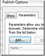
Select Publish Options and the Parameters Tab
When you select Add the Named Range you selected should be available for you
Publish to SharePoint and everything in Excel should be ready for you to use.
Setting up in PerformancePoint
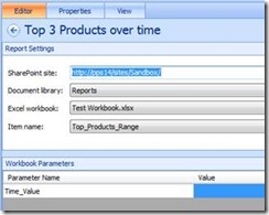
Set up the Excel Report in PerformancePoint the usual way. The Workbook Parameter should be listed automatically. This is the same parameter that you set up in Excel.
The next item you need to setup is the Time Intelligence Filter in this case. We are creating just two ranges one for last 3 Months, and one for the last 6 months.
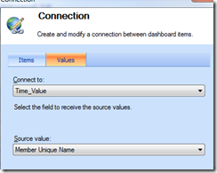
The last think you need to do is hook it together in the Dashboard. Add both the time filter and the Excel Report as components to your dashboard. Use the Member Unique Name as the beginning point and Time_Value as the endpoint.
The end result is that you have dynamic Excel Report that works with the time filter MDX values, or any range values that comes from other filters.
Leif Brenne
Lead Program Manager
Office BI, Microsoft


