Use of hierarchical clustering to predict the end location of a trip
Use of Hierarchical Clustering to Predict the End Location of a Trip
By Beat Schwegler, Partner Catalyst Team
In this case study, our customer needed to predict the end location of a trip so that they could effectively manage their car-sharing fleet. We used Azure ML and Storm to build a model that predicts the end location of individual trips, which customer can then aggregate to most effectively reposition cars as needed to meet expected demand. If you are a developer interested in location hot spots or techniques for hierarchical geofencing, read this case study to understand both model and implementation of these techniques.
Customer Problem
Our customer runs large scale car sharing fleets across multiple cities worldwide. They need to identify locations with high demand to ensure that enough cars are available for pick-up. To plan the fleet repositioning, it is important to predict possible drop-off locations. Together with their demand prediction, this allows the customer to take pre-emptive actions, such as repositioning cars (e.g. through limited time special offers). In this paper we discuss and implement an approach to predict drop-off locations based on one, real-time transmitted pick-up location.
Overview of the Solution
The overall architecture of the solution leverages a real-time data processing pipeline.
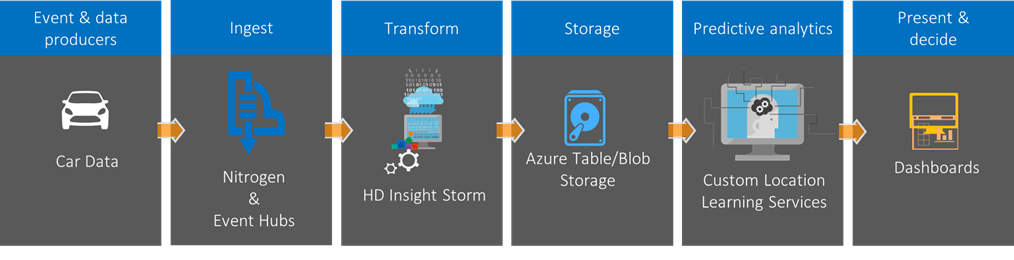
Figure 1: real-time data processing pipeline
The car (or any other device) periodically sends its location which is ingested into the pipeline for further processing. In this solution, we use Storm (https://azure.microsoft.com/en-us/documentation/articles/hdinsight-storm-overview/) to analyze the input stream and generate a summary for each trip, which we store in table storage. Each trip summary contains the following information:
start location, end location, start time, trip duration, driver id
Our approach is based on the assumption that drivers follow certain patterns, such as driving from the train station to the office, or bringing kids to school each weekday morning. The idea is to identify the driver’s most likely drop-off locations based on the current pick-up location.
To implement the location clustering, we created a hierarchical model and computed the cluster that contains the highest number of locations. In such a model, each cluster is divided into four child clusters until we arrive at the required cluster size, the so-called leaf cluster. Each leaf cluster contains its list of locations. To limit the memory footprint and improve performance, we decided not to pre-create the clusters and leaves but to create them only when a location is added to the respective cluster/leaf. Figure 2 to Figure 4 show a representation of the clustering, and a visualization that only clusters containing actual locations are created. The red clusters in Figure 4 highlight the five top leaves (the leaves containing the most locations).
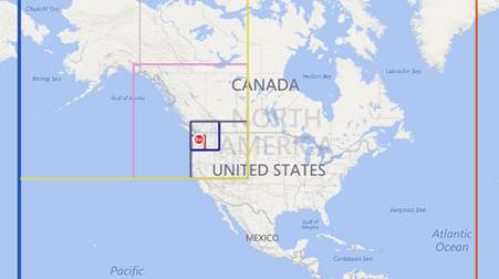 Figure 2: Visualization of clusters (actual locations are in the Seattle area)
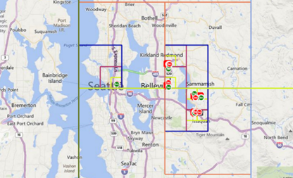
Figure 3: Zoomed visualization of clusters (green pin = start location, red pin = end location)
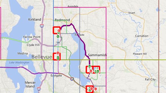
Figure 4: Zoomed visualization of the 5 top locations (the leaves are marked in red)
One issue with a fixed hierarchical cluster is that the actual top location might be located in the intersection of leaves, and therefore won’t be identified by the model (Figure 5).
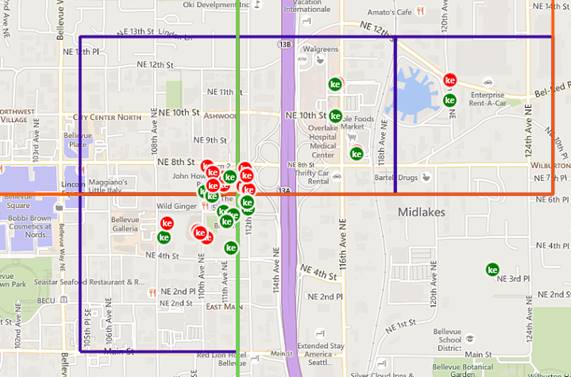
Figure 5: Top cluster is in the intersection of three leaves
To address this issue, we simply created a second model which is shifted by half of the leaf size, both vertically and horizontally. We then query the two models for their top locations and remove intersecting leaves by only taking the one with the highest number of locations (Figure 6).
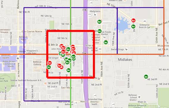
Figure 6: Using a second but shifted model returns the actual intersecting top cluster (the red square)
For the drop-off predictions based on the start location, we perform the following steps:
We load all trips for the particular driver into the model and retrieve all trips that started in the same cluster. For improved accuracy, we can filter trips based on day or time before loading them into the model. The solution could also be extended to run filter queries as part of the top location retrieval, so basically passing a LINQ expression as an argument.
We retrieve all trips that started in the same leaf. In the case no previous trip started in the current leaf, we iteratively query the parent cluster, until we find a trip or reach a cluster level where the prediction becomes irrelevant.
We now iterate over all the trips that started in the same cluster and create a list of leaves where these trips ended. We then count how many of the trips end in a particular leaf and calculate the probability of the prediction.
Limitations: It is clear that this route prediction only works for drivers who follow a specific pattern, such as frequently driving from the train station to the office. Figure 7 shows the performance of a driver which follows a certain pattern: The prediction accuracy progressively increases. After ~40 trips, the model is able to predict around ~60% of end locations with an accuracy of 200 meters.
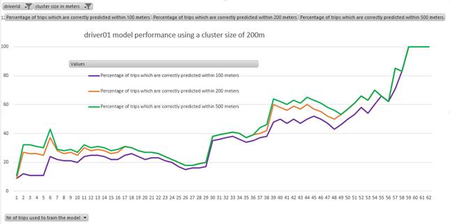
Figure 7: Performance for a driver who follows a regular trip pattern
This is comparison to the second driver (see Figure 8): After only 10 trips, we’re able to predict ~50% of end locations with an accuracy of 200 meters. After around 100 trips, it looks like the driving pattern changes and the accuracy decreases.
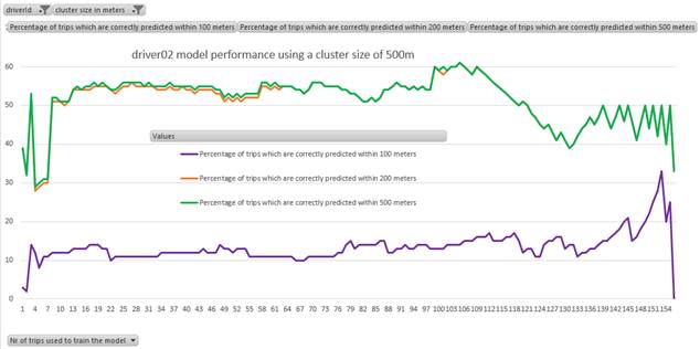
Figure 8: Performance for a driver with changing trip pattern
Implementation
The solution consist of two algorithms: First the hierarchical clustering and second the actual route prediction algorithm (which leverages the clustering for its predictions).
The code for the two algorithms can be found on GitHub: https://github.com/cloudbeatsch/RoutePrediction.
Hierarchical clustering algorithm
The hierarchical clustering algorithm is based on the composite pattern (Figure 9).
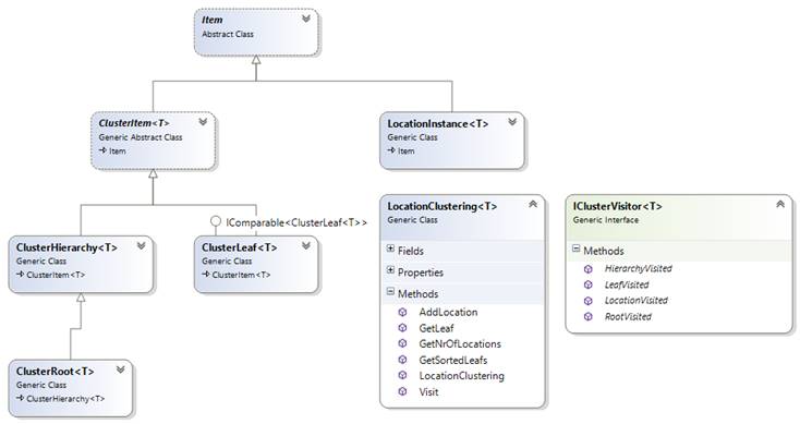
Figure 9: Class diagram - hierarchical clustering algorithm
· LocationClustering represents the service façade and implements the algorithm to query the top location
· Each model consists of a single root cluster of type ClusterRoot
· Each hierarchy level represents a different zoom level and contains one to four child clusters (which are either of type ClusterHierarchy or ClusterLeaf in the case that the minimal cluster size has been reached) (Figure 8)
· Each leaf contains a collection of LocationInstance objects (of which each contains a location object of type T)
· The cluster hierarchy can be traversed using a visitor which implements IClusterVisitor
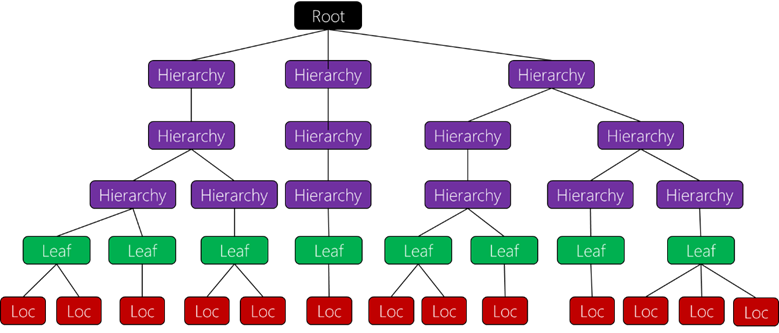
Figure 10: Sample cluster hierarchy
Clustering locations to identify top locations
Using location clustering to identify top locations is straightforward:
1. 1. Create an instance of LocationClustering<T> by typifying the location object and specifying the size of the leaf in meters
var locations = new LocationClustering<string>(200);
2. Add locations using the AddLocation method
locations.AddLocation(latitude, longitude, “<tripId>”);
Locations can be added at any time. This allows the model to learn even after the first top leaves have been queried.
3. 3. Once the locations have been added, just query the top clusters using the GetSortedLeafs method. This returns an enumerable with the requested number of top leaves (the top clusters).
foreach (var leaf in locations.GetSortedLeafs(maxNrTopClusters)) {
foreach (var location in leaf.GetLocations())
{
var tripId = location.LocationObject;
}
}
Predict end locations based on start location
To predict end locations, we build a single cluster per driver using previous trips. We add the start locations and store the trip’s end location as the LocationObject. In the example below, we store objects of type TripSummary (which contains latitude and longitude of the end location):
var locations = new LocationClustering<TripSummary>(200);
locations.AddLocation(startLat, startLon, tripSummary);
Once all the trips have been loaded, the model can be used to predict end locations based on start latitude and longitude. In its essence, this requires the following steps:
1. Retrieve the leaf for the start location. In the case the retrieved leaf contains no trip, we iterate over the parent cluster until we have a cluster which contains at least one trip.
2. For each trip in the cluster, we retrieve its end location leaf and count how many trips end in the same leaf.
3. To calculate the probability of our prediction, we divide the number of locations in a leaf by the total number of locations.
public List<RoutePredictionItem> PredictEndLocation(double startLat, double startLon)
{
var cluster = startLocations.GetLeaf(startLat, startlon);
int clusterLevel = 0;
// check how many start points we have within a cluster
// and iterate through the cluster hierarchy to get at least 1 location
while (cluster.GetNrOfLocations() == 0){
var parent = cluster.GetParentItem();
if (parent != null){
if (parent is ClusterItem<LocationInstance<TripSummary>>){
cluster = parent as ClusterItem<LocationInstance<TripSummary>>;
clusterLevel++;
}
}
}
Dictionary<ClusterLeaf<TripSummary>, RoutePredictionItem> leafs =
new Dictionary<ClusterLeaf<TripSummary>, RoutePredictionItem>();
// create a list of endLocation leafs and count how many times an end location
// is part of the leaf
foreach (var location in cluster.GetLocations()){
ClusterLeaf<TripSummary> leaf =
location.LocationObject.GetParentItem() as ClusterLeaf<TripSummary>;
if (!leafs.ContainsKey(leaf)){
leafs[leaf] = new RoutePredictionItem() {
Lat = leaf.CenterLat,
Lon = leaf.CenterLon,
NrOfEndPoints = 0,
Probability = 0.0 };
}
leafs[leaf].NrOfEndPoints++;
leafs[leaf].Probability = leafs[leaf].NrOfEndPoints /cluster. GetNrOfLocations();
}
var predictions = leafs.Values.ToList();
// sort the predictions on NrOfEndPoints
predictions.Sort();
return predictions;
}
To test the model and measure its accuracy, we split the dataset into a training and a validation set. Now we only load the training data into the model and validate our algorithm by predicting the end locations of our validation dataset. We now simply compare the predictions with the actual values and calculate the distance between them.
Challenges
One challenge we encountered was the creation of trip summaries, basically the extraction of the start and end location from the transmitted data stream. Since GPS data isn’t always accurate, we have to clean the data using different filters to ensure accuracy. To do so, we built a data pipeline and applied different filters (for example, a filter to remove jittering or a filter to recognize one-off measurements). This work will be published in a separate paper.
Another challenge presented was the decimal degrees format of latitude and longitude: Scaling and traversing across the different hierarchy levels is much more intuitive and less error prone when using a projection of metric X and Y axes (e.g. in meters). That’s why decimal degrees are only used at the service boundary, all internal operations are using the projection in meters. The transformation between the different projections have been implemented in a separate library. This geo transformation library can be found on GitHub: https://github.com/juergenpf/Geodesy.
An alternative approach to the proposed solution could be to use SQL Servers’ spatial data capabilities to count start and end locations in predefined geo-fences.
Opportunities for Reuse
The hierarchical location clustering algorithm can be re-used for any solution that needs to identify location hot-spots or requires a hierarchical geo-fencing. The implemented Visitor allows to traverse the hierarchy and enables additional scenarios such as cluster based aggregation or visualization.
The route prediction algorithm represents a simple but yet effective way to predict end points of frequently done trips, and can be used in a variety of different scenarios. The GitHub repository contains a test project which demonstrates route prediction and validation using sample location data.
Beat Schwegler is a Principal Architect on the Partner Catalyst Team based in Switzerland. Beat enjoys working with organizations of all sizes to develop innovative solutions. He calls himself “head in the cloud – feet on the ground” and loves to share his experiences at conferences worldwide. He blogs at www.cloudbeatsch.com.