SP2013/SP2016 - Quick Search Query Performance Data Extraction and Analysis with Excel
Hi Search Folks,
I wanted to share a quick method to extract Search query performance and build your own Analytics around it.
For a start you would need to familiarize yourself to LogParser Studio (LPS). I've published a post to get you started : https://blogs.msdn.microsoft.com/nicolasu/2016/12/20/sharepoint-working-with-uls/
Search Performance
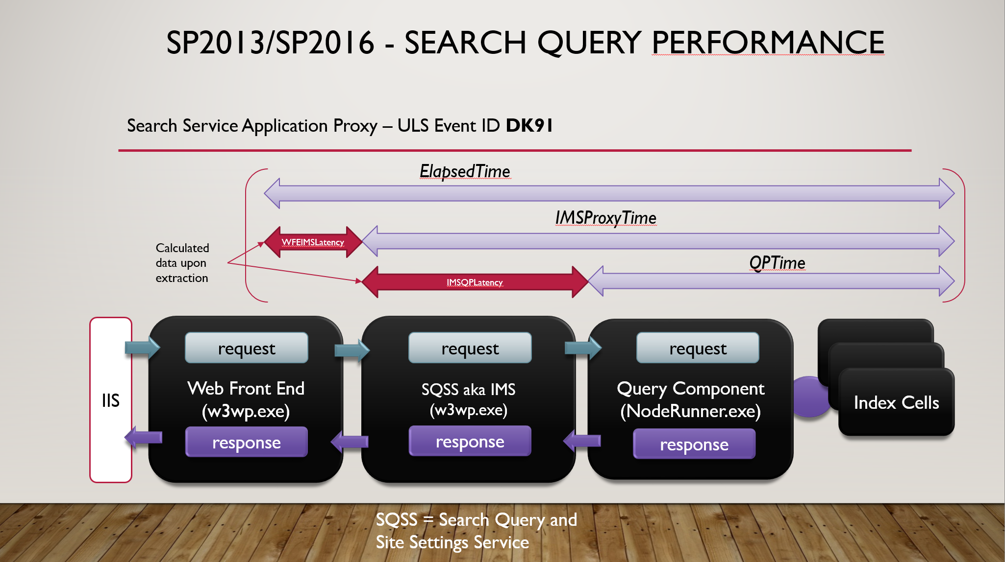
Before diving into the extraction and analysis, I need to point out which tag our Search Performance data will be based upon. The slide below explains at a high level the flow of a Search query.
The ULS entry dk91 is produced by the Web Front End Search Service Application Proxy upon receiving the query response.
High Level Query Flow
Structure of a DK91 Event Message
SearchServiceApplicationProxy::Execute--Id: Elapsed Time: 250 IMSProxyTime 229 QP Time: 214 Client Type CSOM TenantId 00000000-0000-0000-0000-000000000000
All times in DK91 are expressed in ms.
Some counters explaining to do
- "Elapsed Time" : Round trip execution time at the Web Front End level (from the moment the query enters a WFE and returns).
- "IMSProxyTime" : Round trip execution time at the SQSS level (internally named IMS).
- "QP Time": Round trip execution time at the Query Component level. This includes the Index Components exec times.
For convenience of the Analysis, we are adding two new calculated metrics. The below two are useful to highlight resources struggling servers (CPU mostly).
- "WFEIMSLatency" : Latency between the Web Front End and SQSS.
- "IMSQPLatency": Latency between the SQSS and the Query Component.
Time for data extraction
Once you've gained sufficient LPS experience,
- Collect ULS logs files of your SP Web Front Ends (WFE). We will only use those to extract Search Query Performance data.
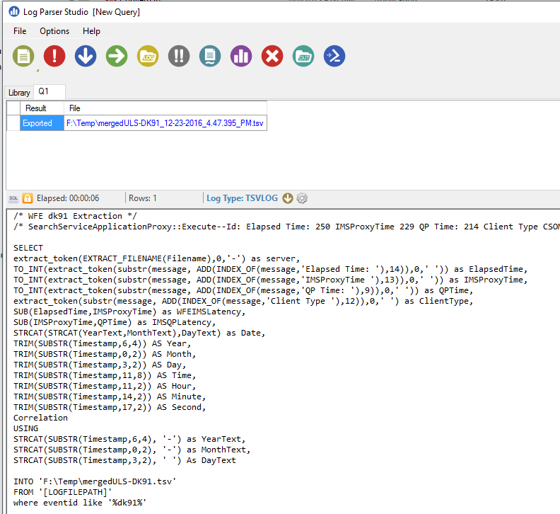
- Create a new Query in LPS
Use the below template. Adapt the output .tsv file name to your convenience.
 /* WFE dk91 Extraction */
/* SearchServiceApplicationProxy::Execute--Id: Elapsed Time: 250 IMSProxyTime 229 QP Time: 214 Client Type CSOM TenantId 00000000-0000-0000-0000-000000000000    ab83b99d-f737-a0bf-1ff7-265cc0d362bc */

SELECT
extract_token(EXTRACT_FILENAME(Filename),0,'-') as server,
TO_INT(extract_token(substr(message, ADD(INDEX_OF(message,'Elapsed Time: '),14)),0,' ')) as ElapsedTime,
TO_INT(extract_token(substr(message, ADD(INDEX_OF(message,'IMSProxyTime '),13)),0,' ')) as IMSProxyTime,
TO_INT(extract_token(substr(message, ADD(INDEX_OF(message,'QP Time: '),9)),0,' ')) as QPTime,
extract_token(substr(message, ADD(INDEX_OF(message,'Client Type '),12)),0,' ') as ClientType,
SUB(ElapsedTime,IMSProxyTime) as WFEIMSLatency,
SUB(IMSProxyTime,QPTime) as IMSQPLatency,
STRCAT(STRCAT(YearText,MonthText),DayText) as Date,
TRIM(SUBSTR(Timestamp,6,4)) AS Year,
TRIM(SUBSTR(Timestamp,0,2)) AS Month,
TRIM(SUBSTR(Timestamp,3,2)) AS Day,
TRIM(SUBSTR(Timestamp,11,8)) AS Time,
TRIM(SUBSTR(Timestamp,11,2)) AS Hour,
TRIM(SUBSTR(Timestamp,14,2)) AS Minute,
TRIM(SUBSTR(Timestamp,17,2)) AS Second,
Correlation
USING
STRCAT(SUBSTR(Timestamp,6,4), '-') as YearText,
STRCAT(SUBSTR(Timestamp,0,2), '-') as MonthText,
STRCAT(SUBSTR(Timestamp,3,2), ' ') As DayText

INTO 'F:\Temp\mergedULS-DK91.tsv'
FROM '[LOGFILEPATH]'
where eventid like '%dk91%'
- This query assumes the ULS file are named following SP standard
SERVERNAME-DATE-TIME.log
for instance SERVER1-20161121-0924.log
If you use a merged ULS log file you can simply modify the query to remove the server field but you will lose the ability to track a misbehaving WFE.
- This query will produce one TSV as you see in the INTO clause.
- Associate the file extension .tsv with Excel for a quick review. The association will result in opening Excel whenever the query is executed and produced the .tsv output file.
Time for Analysis
In this last section I will cover a very quick tip for starting analyzing the Search Performance data. Excel 2016 will be my Analysis tool of preference as it offers powerful yet versatile data visualization.
When the output file is small (<1 Million entries), processing the TSV upon opening in Excel 2016 is enough. When you have over a million entries, you would need to use the Power Query feature within Excel 2016 (previously add on in Excel 2013) which I will cover in a future post.
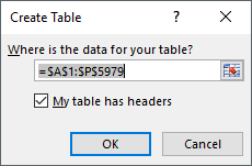
- First convert your raw data into an Excel Table.
- Select the A1 cell and press CTRL+T command
- Once converted to a table, you can create charts, Pivot Table to highlight your Query performance.
I will share below, two simple tips to quickly visualize your data.
Tip #1 : Visualize the response time better with Conditional Formatting.
Conditional Formatting has been in Excel for a while but is a very good starting to get a sense of your performance data.
- Select the entire ElapsedTime column, Click on Conditional Formatting, Choose Data Bars and select the esthetic and color of your choice.
- Repeat the same process for IMSProxyTime and QPTime with different colors.
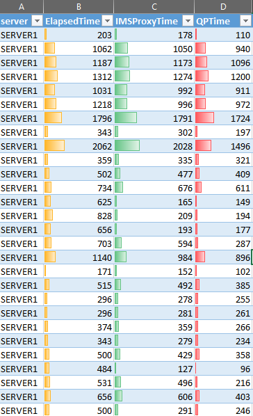
The bars proportions between the 3 columns would give you a feeling of what layers of the Query flow is maybe struggling from time to time.
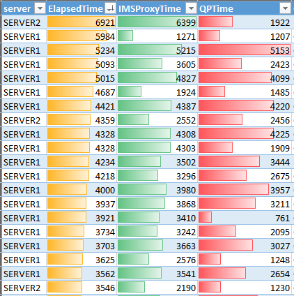
To make it concrete, Sort the Column ElapsedTime from Largest to Smallest
Now validate that when the WFE time is slow all other components are also slow. If not, it will give you a hint that your WFE connectivity with the others layers of the Query flow can degrade. In my example below, the slowest query 6921 ms as reported by the WFE isn't slow on the Query Component (1922 ms) but response time has been lost in between. By sorting you can also spot if a particular server is more impacted by another (i.e. server1 vs server2).
Use Data Bars on WFEIMSLatency and IMSQPLatency to validate the same.
Tip #2 : Create an histogram of Query Component response time distribution (QPTime)
An Histogram on the QPTime will show up the buckets (i.e bins) of Performance and associated frequency. For instance how many queries are taking less than 1000ms, how many between 1000ms-2000ms etc.
- Select the QPTime column
- Click on the Insert ribbon
- Click on Recommended Charts
- Select the Histogram
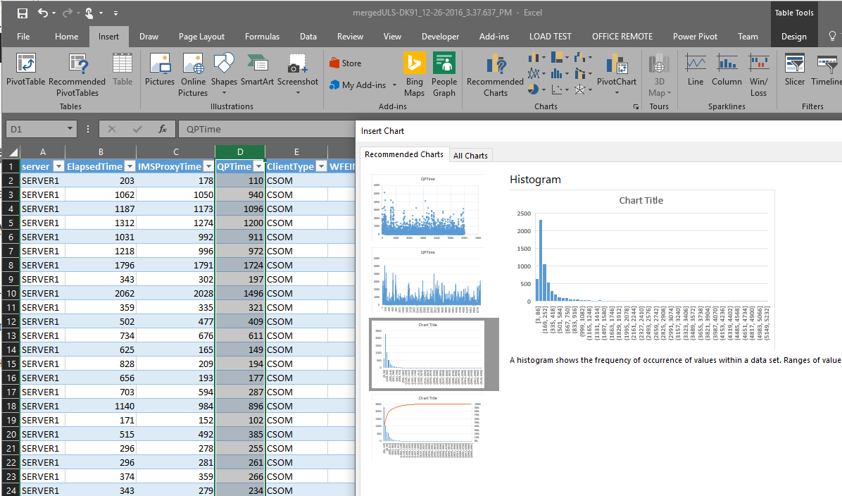
- Press Enter, you will the Histogram
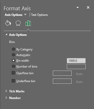
- Now we will modify the x-axis to create more meaningful performance buckets.
- On the histogram chart, right click on the X-Axis,
- In The Axis Options, set Bin width to 1000 (1 second bucket).
- Now set a Chart Title, change the design to your esthetic, set the Data Labels
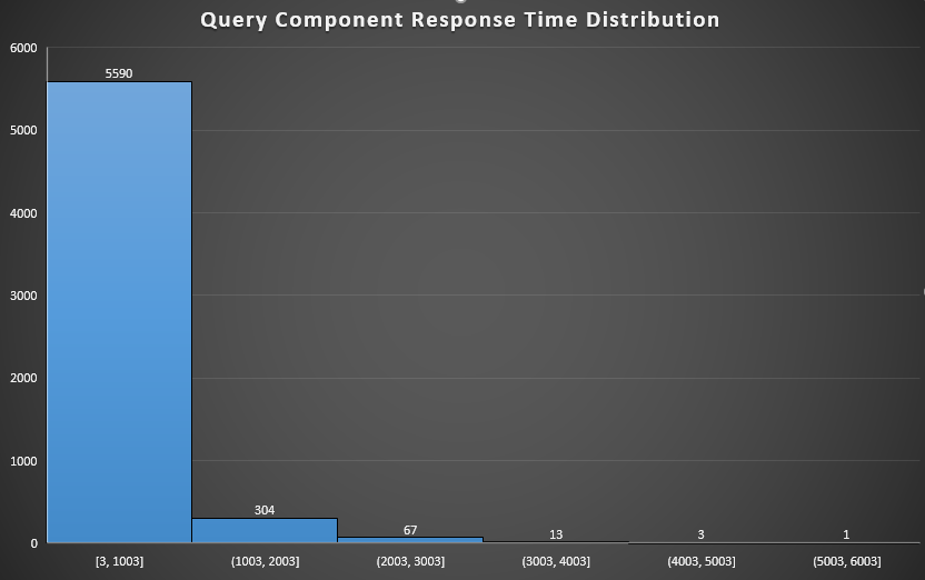
Et voila !
There are plenty of others possibilities of Analysis within Excel 2016, I'd encourage to explore your data once in Excel.
Quite a long post but necessary to provide an end-to-end solution.
Stay in Search