New book: Microsoft Excel 2013 Inside Out

We’re happy to announce the Microsoft Excel 2013 Inside Out (ISBN 9780735669055)by Mark Dodge and Craig Stinson is now available for purchase.

Purchase at The Microsoft Press Store

This supremely organized reference is packed with hundreds of timesaving solutions, troubleshooting tips, and workarounds. It’s all muscle and no fluff. Learn how the experts tackle Excel 2013—and challenge yourself to new levels of mastery. Purchase includes a companion ebook and sample files.

Topics include:

• • • • • • Customizing the Excel workspace
          • Best practices for designing and managing worksheets
          • Creating formulas and functions
          • Performing statistical, what-if, and other data analysis
          • Core to advanced charting techniques
          • Using graphics and sparklines
          • Managing databases and tables
          • Automating Excel with macros and custom functions
          • Collaborating in Excel online, in the cloud, and more
          • Extending Excel

Visit this previous blog post to see the book’s table of contents as well as a description of the book’s audience and an overview of topics.

Here is an excerpt from Chapter 9, “Worksheet formatting techniques.”

CHAPTER 9

Worksheet formatting techniques

When creating a worksheet in Microsoft Excel, you probably don’t ask yourself
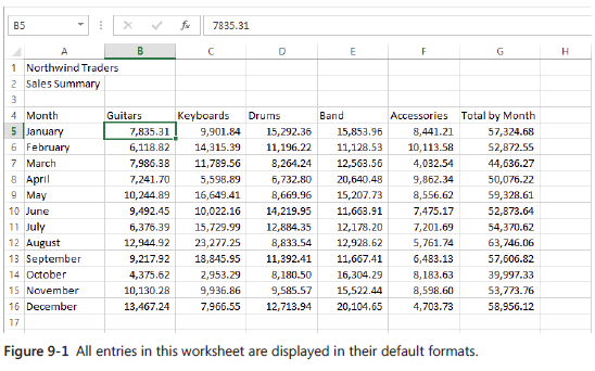
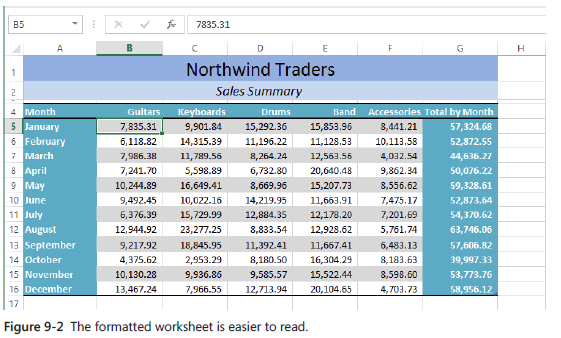
the question, why use formats? But we’ll answer it anyway. Compare Figure
9-1 to Figure 9-2, and we need say no more. Although the data is the same in
both worksheets, the worksheet in Figure 9-2 takes advantage of the formatting features
available in Excel, and as you can see, it’s much easier to read and interpret. In this chapter,
you’ll learn how to apply basic formatting to help turn your data into information.
We also discuss advanced formatting features such as themes, cell styles, and conditional
formatting.

Formatting fundamentals
Worksheet editing involves creating and modifying the content, layout, and organization of data, while worksheet formatting deals with the appearance and readability of that data. With formatting, you can take mind-numbing detail and turn it into information by highlighting the important stuff, adding visual cues and clues, and enhancing overall readability and organization. Be careful, though—over formatting can be as distracting as using none at all. Usually, the goal of a good worksheet is to call attention to the right information, not to showcase Excel’s formatting features (or your mastery of them).
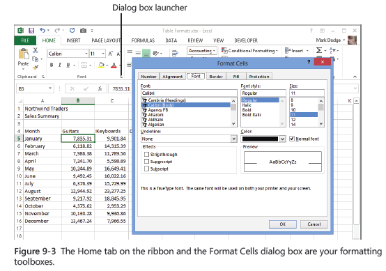
Formatting in Excel is easy: select the cell or range, and use the appropriate buttons and commands on the ribbon to apply formatting. Many of the most often used formatting features appear on the Home tab on the ribbon for quick access, as shown in Figure 9-3. In fact, formatting commands dominate the Home tab; all seven of its ribbon groups include formatting commands (even the Editing group). Figure 9-3 also shows the Format Cells dialog box, which you can access by clicking the dialog box launcher in the Font, Alignment, or Number group on the Home tab on the ribbon. (The dialog box launcher is the small arrow icon to the right of the title in many ribbon groups.)

Here are some fundamental rules of formatting in Excel:
●A formatted cell remains formatted until you remove the format or apply a new format.
●When you overwrite or edit a cell entry, you need not reformat the cell.
●When you copy or cut a cell, the formats applied to that cell travel with it.

Formatting tables

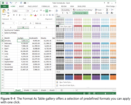
The concept of “tables” in Excel took on fresh meaning with the 2007 release, and it continues through the 2013 release. Tables are special objects in Excel that include many features beyond formatting, but you can use the Format As Table button on the Home tab to apply specific font, border, and fill attributes to all the elements of a table at once. The Format As Table gallery, shown in Figure 9-4, applies predefined combinations of these formatting criteria.

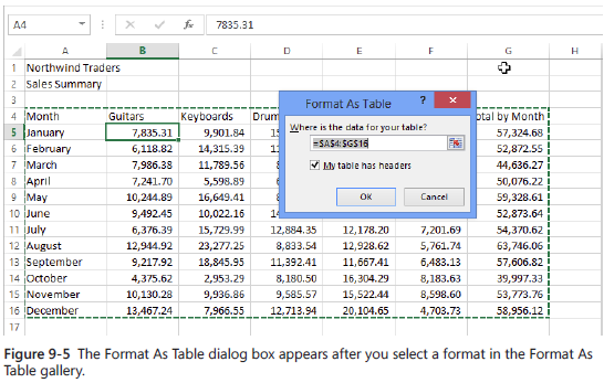
You can apply the Format As Table command to any region of cells (that is, a contiguous block of cells on a worksheet). You select a cell anywhere within the region, click Format As Table, and then select one of the sample table formats from the gallery. When you do, Excel displays the Format As Table dialog box, which lets you adjust the selection, as shown in Figure 9-5.

If your table includes headers (as most do), select the My Table Has Headers check box in the Format As Table dialog box. Excel then selects the entire table automatically and applies the selected table format to it.

Here are a few tips to keep in mind when using Format As Table:
● If you don’t like the way something looks, click the Undo button on the Quick Access Toolbar (or press Ctrl+Z).
● The boundaries of a table are defined by blank rows and columns or the edges of the worksheet. Try adding blank columns or rows around your table to effectively fence off areas you don’t want Format As      Table to touch.
● Select more than one cell before issuing the command, and Format As Table affects only the selected cells.

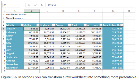
Although Format As Table does a pretty good job with simple tables, you usually need to make a few adjustments afterward. For example, starting with the raw data shown in Figure 9-1, we applied the Table Style Medium 20 format. Figure 9-6 shows the result.

As you can see in Figure 9-6, the title and subtitle in cells A1 and A2 were not part of the table, and therefore were not formatted, so we applied additional formatting manually to arrive at the result shown in Figure 9-2. In addition, we applied number formatting to the cells containing data. Nonetheless, using Format As Table speeds up the formatting process and provides at least one formatting feature that is otherwise unavailable: automatic row and column banding, which was one attribute of the automatic format we applied in Figure 9-6. Another cool part of using Format As Table is the automatic preview feature. After you define a table using the Format As Table command, you can then use the Format As Table gallery to preview other predefined formats. (It doesn’t work on raw data.) Rest the pointer on any format in the gallery, and the associated formatting is temporarily reflected in the table you have already created, but it is not actually applied unless you click.

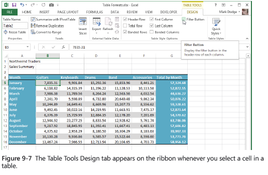
After you create a table, a context-triggered tab appears on the ribbon only when you select a cell or cells within the table. Figure 9-7 shows the Table Tools Design tab.
The Design tab contains formatting commands in the Table Style Options and Table Styles groups. The latter group contains the same gallery as the Format As Table command on the Home tab. In Figure 9-7, we selected both the First Column and Last Column check boxes in the Table Style Options group, which in this particular predefined format applied bold formatting to the fonts in those columns. Also, the Filter Button check box was cleared to unclutter the appearance of the worksheet. (You can always redisplay the filter buttons when you need to massage the numbers; this chapter is all about appearances.) You can select and clear check boxes in this group and view the changes immediately. The Header Row check box actually adds or removes the header row from the table. The Total Row check box adds a double border at the bottom of the table and adds another row containing summary formulas. If you add the summary row, you can select which summary function you want to use by clicking the summary formula in the totals row and then clicking the menu arrow that appears. The menu offers a selection of functions—including Sum (the default), Average, Max, and Min—or you can select More Functions to display the Insert Function dialog box.