New book: Microsoft Excel 2010 Formulas & Functions Inside Out

We’re excited to announce that Egbert Jeschke, Helmut Reinke, Sara Unverhau, Eckehard Pfeifer, Bodo Fienitz, and Jens Bock’s Microsoft Excel 2010 Formulas & Functions Inside Out (ISBN 9780735658028; 1104 pages), ) is now available for purchase! 

You can find the book’s introduction in this previous post.

In today’s post, please enjoy two excerpts – Chapters 3 & 5.

Chapter 3 - “From Numbers to Formulas” - Calculations in Microsoft Excel are achieved through formulas. Formulas are entered differently than other data, although you probably won't notice the difference. The procedure for working with Excel worksheets and working on paper is basically the same, except that when you work on paper you have to write down the initial values and then manually work through each step of the calculation. In Excel, the initial values are called input values, and you specify the algorithms in a formula to produce a result based on the input values.

Chapter 5 - “Functions in Special Operations” - You’ll learn about the use of worksheet functions and in particular how to integrate them with other features of Microsoft Excel to provide a very powerful tool with endless possibilities. Find out what role the functions can play together with names, conditional formatting, and validation.

Chapter 3

Entering Formulas

If an entry in Excel starts with the equal sign (=), the subsequent string is treated as a calculation formula. You can start a formula with the plus or minus sign, but Excel will always add the equal sign at the beginning of the formula.

A formula consists of operands and operators. The operands are the values for the calculation, and the operators are the rules (see Figure 3-1).

Figure 3-1 Operands and operators are the basic elements of a formula.

Operators

The operators that can be used in Excel formulas span the entire range of commonly used symbols. These operators are listed in this section, with the most frequently used first.

Arithmetic Operators

Arithmetic operators are used for basic calculations and return numeric values. Table 3-1 lists the arithmetic operators used in Excel formulas.

Table 3-1 Arithmetic Operators in Excel Formulas

Operator	Operation	Example formula	Result
+	Addition	=15+13	28
–	Subtraction	=104–74	30
/	Division	=42/3	14
*	Multiplication	=5*8	40
^	Exponentiation	=2^8	256
%	Division by one hundred (percent)1	=140%	1.4

¹Like algebraic signs, the percent sign is also an operator.

Sample Files

Use the Arithmetic Operators worksheet in the Chapter03.xls or Chapter03.xlsx sample file. The sample files are found in the Chapter03 folder on the companion website. For more information about the sample files, see the section titled “Using the Sample Files”.

These operators allow you to create formulas in Excel tables by entering the formulas directly into a cell. After you enter a formula, the result is displayed in the cell and the formula is shown as the cell content in the formula bar.

The direct input of numeric values in formulas is also known as entering constants. However, constants are rarely used in formulas. You should avoid constants and replace them with references to input cells that contain the values for the constants. This way you can always update the constant by entering a new value in the cell, and it is always obvious what values have been used in the calculation. The formulas listed in the table use constants only to illustrate the functionality of the operators.

Specifying the Priority of Operations by Using Parentheses

To change the priority of calculation operations, put the expressions you want to calculate first in parentheses. Enter both formulas shown in Table 3-2 in different cells and compare the results to test the functionality of parentheses.

Table 3-2 Result with Parentheses

Formula	Result
=3+8*4	35
=(3+8)*4	44

Note

In a formula, the number of opening parentheses must match the number of closing parentheses. Otherwise, Excel reports an error and highlights the incorrect part of the formula or offers to correct the formula.

SAMPLE FILES

Use the Priority worksheet in the Chapter03.xls or Chapter03.xlsx sample file. The sample files are found in the Chapter03 folder on the companion website. For more information about the sample files, see the section “Using the Sample Files”.

Excel provides input assistance to ensure that you don't lose track of the parentheses and to verify that the number of opening parentheses matches the number of closing parentheses:.

· If you enter a closing parenthesis, the opening parenthesis is highlighted for a few seconds in the formula bar or in the cell.

· If you edit an existing formula and point to one of the parentheses, the matching parentheses are highlighted for a few seconds (depending on your settings).

Priority of Arithmetic Operators

If an expression contains several operators, the priority for calculation is determined by the priority of the operators. You can change the standard priority by using parentheses within a formula. Table 3-3 shows the priority for the operators within an Excel formula.

Table 3-3 Operator Priority

Priority	Operator	Description
1	–	Negation of a value (for example, -34)
2	%	Division of a value by one hundred (percent)
3	^	Exponentiation of a value
4	* and /	Multiplication and division
5	+ and –	Addition and subtraction

You might remember the old arithmetic rule, PEMDAS, which can help you when you are in doubt.

Note

If a formula contains operators with the same priority, Excel calculates the formula from left to right.

Comparison Operators

Use the comparison operators to compare values, text, or cells. These expressions are often used in logical functions; a common example is IF(). The result is always a logical value (Boolean value). Table 3-4 lists all of the Boolean operators and demonstrates them with sample formulas.

Table 3-4 Boolean Comparison Operators

Operator	Operation (comparison)	Sample formula	Result
=	Equal to	=5=8	FALSE
<	Less than	=5<8	TRUE
>	Greater than	=5>8	FALSE
<=	Less than or equal to	=5<=8	TRUE
>=	Greater than or equal to	=5>=8	FALSE
<>	Not equal to	=5<>8	TRUE

SAMPLE FILES

Use the Comparison Operators worksheet in the Chapter03.xls or Chapter03.xlsx sample file. The sample files are found in the Chapter03 folder on the companion website. For more information about the sample files, see the section “Using the Sample Files”.

The & Text Operator

In some cases, you might want to combine the results from several formulas or cells in a single cell. For this task you use the & (ampersand) operator. If you connect two values of any type with the ampersand, the result always has the Text data type. In other words, Excel converts number values automatically into text. This way you can use the text operator to include two number values as text in one cell. However, you cannot use the resulting string directly for other calculations.

Note

If you use text instead of a cell reference in a formula, you must put this text in quotation marks. You don't have to put numbers in quotation marks. Quotation marks are also not necessary if you use references to cells, which can contain any data type.

To connect the content in cells A1 and A2 by using the text operator, enter the following formula:

=A1&A2

The text operator connects the contents of the two cells without a space in between them. To include a space between the values, you must use quotation marks. If you want a space between the values in cell A1 and cell A2, use the following formula:

=A1&" "&A2

SAMPLE FILES

Use the Text Operator worksheet in the Chapter03.xls or Chapter03.xlsx sample file. The sample files are found in the Chapter03 folder on the companion website. For more information about the sample files, see the section “Using the Sample Files”. Figure 3-2 shows the content of this worksheet.

Figure 3-2 Text operator examples you find in sample file.

Reference Operators

With reference operators, you can pass cells or cell ranges to a formula or function for calculation. The following operators are available:

· Range separator : (colon). Creates a reference to all cells between two references, including the reference cells themselves; for example, B3:B20

· Connection operator , (comma). Allows the connection of several cells or references in an expression; for example, SUM(B3:B20,D3:D20)

· Intersection operator (space). Creates a reference to cells that occur in both ranges that are referenced; in other words, the cells are the intersection of both ranges—for example, B7:D7 C6:C8

The Range Operator

A range is an area of a worksheet consisting of cells next to and/or below each other. If two cell references are connected with a colon, these references together with the cells in between form a range. Ranges can have different sizes and shapes. In functions, a range is an argument independent of its size.

Possible Range References

Range references are easily specified. Figure 3-3, shows all of the possible variations.

Figure 3-3 Possible range shapes and syntaxes to use in formulas.

The ranges shown demonstrate the following rules for range reference syntax:

· For a range spanning several columns and rows, the cell in the upper-left corner is connected with the cell in the lower-right corner, as in B3:D10.

· For a range spanning one row, the left cell is linked with the right cell, as in B13:F13.

· For a range spanning one column, the upper cell is linked with the lower cell, as in F2:F9.

References to Entire Columns or Rows

If you want to reference columns or rows from the first to the last cell, use the references listed in Table 3-5. You can create references for other columns and rows based on the references in this table.

Table 3-5 Syntax for References to Entire Columns or Rows

Reference to	Syntax
Entire column E	E:E
Entire row 7	7:7
All rows from row 2 to row 5	2:5
Entire worksheet	A:XFD or 1:1048576

The references for the entire worksheet in Table 3-5 are only valid in Excel 2007 and Excel 2010, because these versions have extended row and column limits. You can find more information in Appendix C.

References can be used in other worksheets and workbooks. Be careful not to reference a cell in a formula that already references that cell, because you will create a circular reference. See the section "What is a Circular Reference?" later in this chapter for further information.

The Connection Operator

You can pass nonadjacent cells to a function for calculation by using a connection or union operator. The connection operator is the comma (,). If you use the connection operator to pass several cells to a function, each cell reference that is separated from another by a comma is treated as a separate argument.

If you wanted to add the three ranges shown earlier in Figure 3-3, you would have to specify each cell group in the SUM() function. The function would have three arguments separated by commas:

=SUM(B3:D10,F2:F9,B13:F13)

The Intersection Operator

The intersection operator is rarely used but should be included in this list. With the intersection operator (the space), you define a reference to the cells shared by several different references. In other words, an intersection in Excel describes the values in the area where two or more ranges overlap.

Figure 3-4 Simple example of an intersection.

The intersection shown in Figure 3-4 is where the ranges B2:E11 and C8:G14 overlap. In a formula or function, this intersection would look like this: B2:E11 C8:G14.

The result of the intersection is called an explicit intersection. The values in the cells in the explicit intersection are added up with the following formula:

=SUM(B2:E11 C8:G14)

Intersections are mostly used in the context of range names and are rarely used as pure cell references.

References in Formulas

As mentioned at the beginning of this chapter, the use of constants in formulas defeats the purpose of a spreadsheet. When you use constants, you have to change the formula each time a value changes.

The content of a cell is handled through a cell reference. A reference tells Excel which cell contains the values used in a formula (see Figure 3-5).

Figure 3-5 Using cell references to multiply the day rate by days.

When you enter references, make sure that the formula doesn't contain spaces.

Note

Formulas are not case sensitive. Excel converts all references from lowercase to uppercase if the syntax of the formula is correct. If it is not, check your entry for syntax and typing errors.

You will find it easier to enter cell references by selecting the cell or cell range you want to use rather than typing it. To enter a formula, perform the following steps:

1. Type the equal sign.

2. Enter any function name, parenthesis, or other character with which a formula can begin.

3. Select the cell or cell range you want to include in the formula as the cell reference. The selection is marked by a dashed line, and the cell reference appears in the formula.

4. Enter the operator or another part of the formula.

5. Select other required cells or ranges.

6. Repeat steps 2 through 5 until the formula is complete.

7. Press the Enter key to complete the formula.

Cell references allow you to use all the advantages offered by a spreadsheet. You can create any number of calculation schemes and change a scheme to get different results.

This means that you only have to create a calculation scheme once and can use it for similar calculations over and over again. In the table in Figure 3-6, you can change the values in columns B and C to immediately get the result in column D.

Figure 3-6 The formula containing cell references can be copied in the cells below.

Another advantage of using cell references in a formula is that you can copy the formula by dragging the fill handle down. In this way you create all of the required calculations within seconds, which would not be possible if you were using constants.

SAMPLE FILES

Use the Relative Reference worksheet in the Chapter03.xls or Chapter03.xlsx sample file. The sample files are found in the Chapter03 folder on the companion website. For more information about the sample files, see the section “Using the Sample Files”.

Relative References

If you copy the formula shown in Figure 3-6 by dragging the fill handle down, you get the correct result for each line. This is because Excel adjusts the references in the formula by using the current row number. However, this only works because the row number in the formula is relative.

Consider a relative reference as the relation between two cells. The relation—not the literal syntax of the reference—is copied.

The formula in cell D3 in the table shown in Figure 3-6 would read like this: "Take the value in the cell two columns to the left in the same row (=B3) and multiply (=B3*) this value by the value in the cell one column to the left in the same row (=B3*C3)."

Caution

The following applies when you are copying a formula containing a relative cell reference:

· If you are copying horizontally, the column references change according to the location.

· If you are copying vertically, the row references change according to the location.

Absolute References

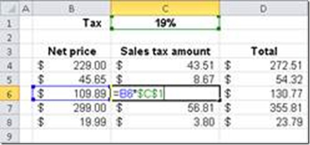
An absolute reference is the counterpart to a relative reference. An absolute reference is a cell reference that doesn't change when it is copied or filled. You use absolute references to anchor a reference in a formula to a particular cell. Assume that you want to calculate the sales tax for several net prices, and the sales tax rate is entered in a particular cell. You need to be able to copy the formula you created (see Figure 3-7).

Figure 3-7 Initial situation with the formula in cell C4.

The formula entered in cell C4 calculates the sales tax for the net price in cell B4. The formula is:

=B4*C1

If you copy this formula to the cells below, you get the wrong results because the relative cell references change. Cell C6 even displays the error message #VALUE!. Because cell C3 contains the text "sales tax amount" the #VALUE! error is generated.

When you analyze the formula in cell C4, you'll see that the reference to the sales tax should not be changed. To ensure that the sales tax doesn't change, enter a dollar sign ($) before the column (C) and the row (1) references. Now this cell reference won't change when copied or filled and is called an absolute reference in Excel.

The formula in cell C4 in the table shown in Figure 3-7 should read:

=B4*$C$1

If you fill the range with this formula starting at cell C4 and copy the formula in the cells below it, the entire table shows the correct results (see Figure 3-8).

Figure 3-8 Correct results due to the absolute cell reference to cell $C$1.

SAMPLE FILES

Use the Absolute Reference worksheet in the Chapter03.xls or Chapter03.xlsx sample file. The sample files are found in the Chapter03 folder on the companion website. For more information about the sample files, see the section “Using the Sample Files”.

Mixed References

Actually, you didn't need an absolute reference to copy the formula in the example shown in Figure 3-8. Because you copied the formula in the same column, the column reference didn't have to be absolute. This leads us to mixed references which are, as the name implies, a mix of relative and absolute references.

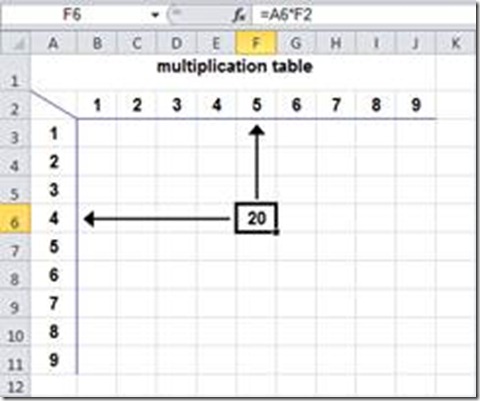
Assume that you want to create a multiplication table. The calculation method to use is obvious. Look at the formula for cell F6 in the formula bar of the table shown in Figure 3-9: =A6*F2. In B3, the formula would be: =A3*B2. As you probably can guess, the formula doesn't have to be rewritten for each cell.

Figure 3-9 A multiplication table as an example for using mixed references.

If you could lock the column or row reference, you could copy the formula created in cell B3 in the table shown in Figure 3-9 to the cells below and to the right. The solution:

· You have to lock the column reference for the values in column A to copy the formula horizontally and to always use the values in column A. The row reference for the values in column A has to remain relative so it can be adjusted when copied vertically. The result is the cell reference $A3.

· For the reference to the values in row 2, it is the other way around. The column reference has to remain relative and the row reference has to be locked with the $ sign. This way, the reference to the row is not changed when the formula is copied vertically, but the column references are adjusted when it is copied horizontally. This leads to the following formula for cell B3:

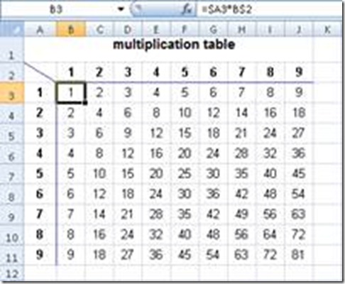
=$A3*B$2

Try this in your table. You will always get the correct results (see Figure 3-10).

Figure 3-10 The results are correct when mixed references are used.

SAMPLE FILES

Use the Mixed Reference worksheet in the Chapter03.xls or Chapter03.xlsx sample file. The sample files are found in the Chapter03 folder on the companion website. For more information about the sample files, see the section “Using the Sample Files”.

The basic principle is this: For a mixed reference, the part after the dollar sign is locked and cannot be changed when copied. Remember these two rules:

· To always apply the values in a certain column, lock the column reference with the dollar sign.

· To always apply the values in a certain row, lock the row reference with the dollar sign.

You can press the F4 key to change the reference type. Click into the cell reference in a formula and press F4 several times. Each time you press F4, the syntax changes (relative to absolute to mixed to relative, and so on).

Finally, we want to mention a new feature in Excel 2007/Excel 2010: In list ranges marked as Table, you’ll find a new syntax for (relative) references, as in the following example:

=[@Price]*[@Quantity]

The example multiplies the values in the columns with the Price and Quantity headings for each line. If you enter a formula in row 1, Excel fills the adjacent empty cells below with the new formula.

What Is a Circular Reference?

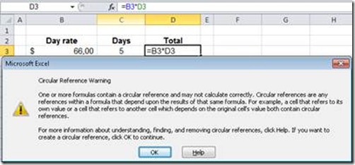
Circular references are mostly generated by input errors. A circular reference is a reference to a cell containing the formula, in other words, a reference to itself. Excel cannot resolve formulas with a circular reference. Instead you receive the message shown in Figure 3-11.

Figure 3-11 Wrong input in cell D3 and error message.

If you click OK in the error message, the circular reference toolbar appears in the table window of Excel 2003 (see Figure 3-12).

Figure 3-12 The circular reference toolbar in Excel 2003.

You can use the circular reference toolbar to iterate through the cells within the circular reference. Use the Trace Dependents and Trace Precedents buttons to see what caused the problem.

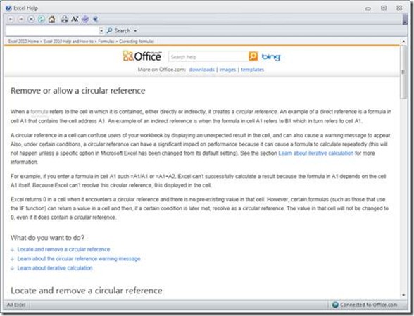
If you click OK in the circular reference warning in Excel 2010, a help window shows instructions on how to handle circular references (see Figure 3-13).

Figure 3-13 Excel 2010 help for circular references.

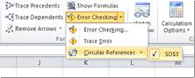
In Excel 2007/Excel 2010, you can find the search and remove options for circular references on the ribbon, on the Formula tab. In the Formula Auditing group, click the Error Checking and then the Circular References button. Then click the displayed references (see Figure 3-14). However, here (and in the status bar), only the circular reference entered last is displayed.

Caution

If you close the warning and the help window and don't correct the circular reference, no other warning is displayed when you enter another formula with a circular reference in a cell. However, the status bar shows circular references. So correct circular references immediately, because you might forget later.

Figure 3-14 Finding circular references in Excel 2007/Excel 2010.

Inside Out More about Circular References

Excel cannot calculate all open workbooks automatically if one workbook contains a circular reference. You have to remove the circular reference or you can calculate each cell included in the circular reference by using the results of the previous iteration. If you don't change the default settings for iterations, Excel ends the calculation after 100 iteration steps or if the values in the circular reference change by less than 0.001 between two iterations (depending which happens first).

Chapter 5

Functions in Names

Using Excel functions in names can extend a simple naming facility and offer possibilities for specifying arguments in these functions. In Chapter 2, “Using Functions and PowerPivot,” you learned about the different syntaxes for references. In addition to basic relative, mixed, and absolute cell references, the use of names for functions provides further possibilities.

A name can be used for

· a reference

· a constant

· a formula

Querying Current Information

You can use an information function (see Chapter 10, “Lookup and Reference Functions”) to query the path, file name, and sheet name of the current saved workbook. The workbook must be saved, otherwise an empty string ("") will be returned. The formula is:

=CELL("filename")

but the function returns all the information in a single string; for example:

C:\Excel-Functions\Chapter05\[Chapter05_Names.xls]Fct_Names

The text functions in Chapter 8, “Text and Data Functions,” provide a method to isolate the individual sections of information; this is often called parsing. This approach can be useful if you want to insert this information directly into the sheet rather than using the text modules &[Path], &[File], and &[Tab], which are available in the worksheet header or footer sections.

Querying the Path of the Current Workbook

The path of the workbook is at the beginning of the string and ends at the left bracket “[“. To isolate the string to the left of this point, the following syntax is used:

=LEFT(CELL("filename"),FIND("[",CELL("filename"))-1)

The FIND() function calculates the position number of the left square bracket, and LEFT() determines the string up to the position of this bracket. The following steps describe how these functions are used:

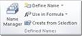
1. In Excel 2007/Excel 2010 on the Formulas tab, click the Define Name icon (see Figure 5-1). In Excel 2003, select the Insert/Names/Define menu command.

2. Enter the text Path in the Name text box (Excel 2007/Excel 2010) or New Name text box (Excel 2003).

3. Enter the formula shown earlier in this section in the Refers To field, and click OK (Excel 2007/Excel 2010) or Add (Excel 2003).

Figure 5-1 The Defined Names group on the Formulas tab in Excel 2007/Excel 2010.

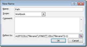
Figure 5-2 shows the New Name dialog box in Excel 2007/Excel 2010, which is different from the old Define Name dialog box.

Figure 5-2 Entering a calculation for the name Path.

Querying the File Name of the Current Workbook

Extracting file names requires a little more effort. You need to query the string between the square brackets:

=MID(CELL("filename"),FIND("[",CELL("filename"))+1,FIND("]",CELL("filename"))-(FIND("[",CELL("filename"))+1))

Identify the file name with the MID() function, using the FIND() function to locate the [ character to determine the start_char parameter, and combine this with the FIND() function that locates the ] character to determine the num_chars parameter. Here’s how you use this formula:

1. Select the Define Names command and enter File name in the Name box.

2. Enter the formula just shown in the Refers To field, and click OK (or Add, in Excel 2003).

Querying the Current Sheet Name

Isolate the current sheet name with the RIGHT() function or the MID() function. If you use the CELL() information function, make sure that the sheet name displays the tab label on each sheet by defining the optional second argument. which must contain a reference to any worksheet cell. Use the INDIRECT() function for this worksheet cell reference so that Excel doesn’t attach the sheet name to references (for example, Table1!A1). Here we use the MID() function because it is shorter than using the alternative RIGHT() function:

=MID(CELL("filename",INDIRECT("A1")),FIND("]",CELL("filename", INDIRECT("A1")))+1,255)

Identify the sheet name with the MID() function. The Start_num argument is set by determining the position of the right bracket with the FIND() function. Use the number 255 for the num_chars argument. This covers names up to the maximum allowed length. The following steps show how to use this formula:

1. Select the Define Names command. Enter Sheet name in the Name box.

2. Enter the formula just shown in the Refers To field, and click OK or Add (for Excel 2003).

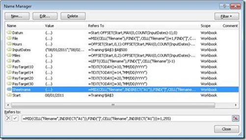
Excel 2007 introduced a new tool: the Name Manager (see Figure 5-3). This provides a much improved facility for defining, editing, and managing the names used in a workbook.

Figure 5-3 The Name Manager in Excel 2007/Excel 2010 provides significantly better options for working with names.

Payment Targets as “Text Modules”

Assume that your company uses different payment targets for billing. These targets range from immediate payment to due dates in 10, 14, 20, or 30 days. To specify a payment target, you should enter a term that provides the date in a text format:

1. Select the Define Names command. Enter PaymentTarget10 in the Name box. Then enter the formula

=TEXT(TODAY()+10,"MM/DD/YYYY")

in the Refers To field and click OK.

2. Repeat these steps to create the second name, PaymentTarget14. Enter the formula

=TEXT(TODAY()+14,"MM/DD/YYYY")

in the Refers to field and click OK.

3. Create the names PaymentTarget20 and PaymentTarget30 with the formulas

=TEXT(TODAY()+20,"MM/DD/YYYY")

and

=TEXT(TODAY()+30,"MM/DD/YYYY")

You can now use the formula ="Please pay the invoice amount by " & PaymentTarget20” to set the payment target in an invoice form by specifying the name—PaymentTarget10, PaymentTarget14, and so on—in the formula.

Sample Files

Use the Fct_Names worksheet in the Chapter05_Names.xls or Chapter05_Names.xlsx sample file. The sample files are found in the Chapter05 folder on the companion website. For more information about the sample files, see the section titled “Using the Sample Files”.

Dynamic Range Names

The following example demonstrates how powerful names can be: Assume that you have a list to which entries are added on a daily or weekly basis. When you evaluate the list, you want the calculation to expand automatically to cover the additional entries. How can you achieve this?

Note

Another example of using dynamic range names can be found in Chapter 2, in the section “Using Database Functions.”

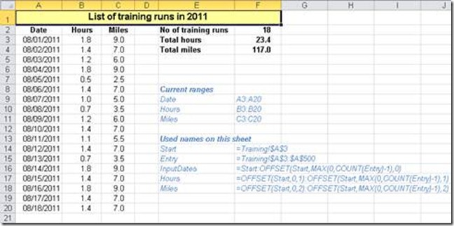
Assume that each day you enter fitness training data into a table. Column A contains the date, column B the time taken, and column C the distance covered (see Figure 5-4).

Figure 5-4 The names point to the extended range if new values are entered

The maximum number of rows in the worksheet will be 367 (including the title row and 366 leap year days) if each calendar year has its own worksheet. Create a name that will reference the maximum used range.

The solution lies in how the names are assigned:

1. Give the date range A3:A500 the name Entry.

2. Specify the name Start for cell A3.

3. Specify the name InputDates. Enter the following formula in Refers To:

=start:OFFSET(start,MAX(0,COUNT(Entry)-1),0)

4. For the name Hours use the reference

=OFFSET(start,0,1):OFFSET(start,MAX(0,COUNT(Entry)-1),1)

5. For the name Miles use the reference

=OFFSET(start,0,2):OFFSET(start,MAX(0,COUNT(Entry)-1),2)

To identify the dynamic range, you can use the function OFFSET(reference, rows,columns,height,width) to return a reference that is offset from a specified reference. In this case, the range starts in the row defined by the name Start, with the appropriate column selected by the Offset parameter. The MAX function identifies the number of numeric entries in the Entry range and is used in the OFFSET function to extend the range out to this point.

It is important to remember that the names Hours and Miles are based on the entries made in the Date column and thus this example relies on a date being entered for each line of information.

Note

The functions associated with names are not displayed in the Name box and in the Go To dialog box. To check these names, click in the Name box and enter the name or press F5 to open the Go To dialog box, enter the name Hours or Miles in the Reference field, and click OK.

Add new entries to the data to the test the ranges. Press the F5 key to open the Go To dialog box and locate the reference again. You will notice that the name now points to the extended range, and the calculated values for sessions, time, and distance are based on the extended range.

Sample Files

Use the Training worksheet in the Chapter05_Names.xls or Chapter05_Names.xlsx sample file. The sample files are found in the Chapter05 folder on the companion website. For more information about the sample files, see the section titled “Using the Sample Files”.

A dynamic name can be invaluable for defining a dynamic chart.

Functions for Conditional Formatting

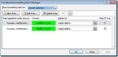
Excel 2003 offered a range of conditional formatting options with up to three rules. This feature has been greatly improved in Excel 2007/Excel 2010, extending the number of rules without any limit. Also, in addition to standard formatting, you now have a range of color scales, data bars, and icons to choose from. There is also a Rules Manager, offering a much improved method of defining and managing the rules (see Figure 5-5).

Figure 5-5 The Rules Manager for conditional formatting in Excel 2007/Excel 2010.

In addition to simple data range selections, conditional formatting can also be applied to formulas.

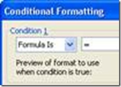
In Excel 2003, select Formula Is in the left side of the Conditional Formatting dialog box (see Figure 5-6) and enter the formula in the field to the right. The formulas must return the value TRUE or FALSE. If the formula returns TRUE, the formatting is applied according to your settings.

Figure 5-6 In Excel 2003, select Formula Is instead of Cell Value Is.

In Excel 2007/Excel 2010, on the Home tab, click the Conditional Formatting button and select New Rule. Then select the Use A Formula To Determine Which Cells To Format rule type.

The ability to use a formula to set conditional formatting, together with the range of functions available in Excel, and now the unlimited number of rules in Excel 2007/Excel 2010, the possibilities are endless. The following examples explore just a few of the capabilities.

Note

The Chapter05_CF.xlsx workbook in Excel 2007/Excel 2010 file format, and the additional New in Excel 2007|2010 sheet show the new possibilities based on the following temperature example.