New book: Microsoft PowerPivot for Excel 2010: Give Your Data Meaning

We’re excited to announce that Marco Russo and Alberto Ferrari’s Microsoft PowerPivot for Excel® 2010: Give Your Data Meaning (ISBN 9780735640580; 416 pages) is now available for purchase!  

You can find the book’s Contents at a Glance and an excerpt from the Introduction this previous post.

In today’s post, please take a look at Chapter 2, “PowerPivot at Work.”

Chapter 2

PowerPivot at Work

We are now going to introduce some of the most interesting features of Microsoft SQL
Server PowerPivot for Excel. The goal of this chapter is to show the most frequently used
PowerPivot features for transforming a simple Excel workbook into a complex report that
helps you perform analysis on data. This is not yet the place for more advanced topics,
such as the DAX programming language or complex relationships. Nevertheless, after you
read this chapter, you will be able to perform complex analysis on a relational database
and—we hope—still feel the need to go forward in your reading to discover the most
advanced uses of PowerPivot.

Please note that we sometimes refer to the end user or the user experience as if we think that your
PowerPivot workbook might be used by somebody else. To make a good report, you always
need to think in this way. Even if you are the only user of a specific report, a user-friendly report
is easier to read and update even after some time has passed since its creation.

Using the PivotTable to Produce Report

Let us start with a very simple report, based on the same three tables that you loaded in the
previous chapter: Sales Order Header, Sales Order Detail, and Product.

If you create a PivotTable with PowerPivot and put OnlineOrderFlag and SizeUnitMeasureCode
on the Report Filter pane, Size on Column Labels, Color on Row Labels and the OrderQty as
the value to sum up, you end up with the report shown in Figure 2-1, which you can find in the
workbook named CH02-01-FirstSample.xlsx in the companion content.

Figure 2-1 A simple report using PowerPivot.

Before analyzing more advanced features, let us recall briefly what is going on:

• The OnLineOrderFlag, coming from the SalesOrderHeader table, is a TRUE/FALSE value.
  PowerPivot found only two possible values for it, so it has been able to fill the combo
  box of the filter with the values True and False. By choosing True, you selected only the
  orders placed online.
• The same process happened for the SizeUnitMeasureCode, this time coming from the
  Product table. It can contain only two distinct values (empty and CM). You have selected
  CM as the measure unit for the size.
• Placing Color on the rows, Size on the rows, and finally OrderQty as the value,
  PowerPivot analyzed all the rows containing the value (which is OrderQty, contained
  in the SalesOrderDetail table). Then it followed the relationship between Order Detail
  and Products and filtered out all the rows from the detail that do not satisfy the filter
  condition. In the meantime, it removed all the rows that do not satisfy the condition
  on the OrderHeader table, which contains the OnlineOrderFlag.
• Having detected the set of rows that you want to analyze, PowerPivot followed the relationship
  between SalesOrderDetail and Product to find out the color and the size of each
  product sold, summarized up all the quantities, and displayed the final PivotTable.

Do not worry if the process described here is not perfectly clear; it will become easier to
understand as you continue reading, thanks to the many examples we are going to provide.
But remember this important point: the presence of relationships is essential for PowerPivot
to detect the set of rows it must take into account from the source tables.

Figur e 2-2 Wrong display of numbers if format strings are applied to the PivotTable.

In the next chapters, we spend several pages in the analysis of different kinds of relationships
and how to master them. Nevertheless, before diving into complex analysis, let us solve some
minor problems in this sample report to make it more appealing and a smoother introduction
to all of the PowerPivot features.

Formatting Numbers

Even if the report shown in Figure 2-1 contains interesting information, it has a problem: it lacks
a format for numbers. In Excel worksheets, the formatting of numbers is one of the functions of
the worksheet itself. So, to format the numbers properly, you select the data area of the report
and choose a proper formatting. If you follow this procedure in a PivotTable, the first result is
not very appealing, as you can see in Figure 2-2.

Figure 2-2 Wrong display of numbers if format strings are applied to the PivotTable.

Because you applied the formatting after you created the PivotTable, none of the columns
were large enough to accommodate the new representation of numbers, which now contain
dots and commas, resulting in larger columns. You can solve this easily by resizing all the
columns. Nevertheless, if you decide to change the measure displayed and use a different
one (for example, ListPrice), you probably need a different format and different column
sizes, and you probably have to resize the entire worksheet.

The correct procedure to follow is to use the PivotTable field settings to define a number format
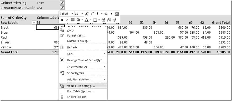
for the OrderQty column. To perform this, you can right-click inside a cell containing the
OrderQty value and, from the menu, choose Value Field Settings, as you can see in Figure 2-3.

Figure 2-3 The Value Field Settings menu.

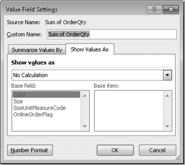
This option opens the Value Field Settings dialog box, shown in Figure 2-4, which contains
many options. We are interested, for now, only in the number format, which you can view
by clicking the Number Format button.

Figure 2-4 The Value Field Settings dialog box.

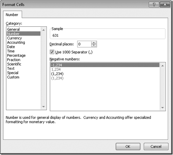
The Format Cells dialog box (see Figure 2-5) lets you choose a number format for the column in
this PivotTable.

Figure 2-5 The Format Cells dialog box.

When you choose the number format you want (in this case, we have selected a number format
with a thousand separator and no decimal places), the PivotTable resizes all the columns
automatically, as you can see in Figure 2-6.

Figure 2-6 The PivotTable correctly resized.

This procedure applies number formatting to the current PivotTable only. If the same column is
used somewhere else in other PivotTables, your choice in this PivotTable does not affect them.
Please note that, if you change the measure shown, you must repeat the procedure to
determine the number format of the new column used.