Building Mission Critical Systems using Cloud Platform Services
Overview
Mission critical systems will often have higher SLA requirements than those offered by the constituent cloud platform services. It is possible to build systems whose reliability and availability are higher than the underlying platform services by incorporating necessary measures into the system architecture. Airplanes, satellites, nuclear reactors, oil refineries and other mission critical real world systems have been operating at higher reliabilities in spite of the constant failures of the components. These systems employ varying degrees of redundancy based on the tolerance for failure. For instance, Space Shuttle used 4 active redundant flight control computers with the fifth one on standby in a reduced functionality mode. Through proper parallel architecture for redundancy, software systems can attain the necessary reliability on general purpose cloud platforms like Microsoft Azure. The SLA numbers used in this document are theoretical possibilities and the real SLA numbers depend on the quality of the application architecture and the operational excellence of the deployment.
Reliability of Software Systems
Any system that is composed of other sub systems and components exhibits a reliability trait that is the aggregate of all of its constituent elements. This is true for airplane rudder control, deployment of solar panels in a satellite, or the control system that maintains the position of control rods in a nuclear reactor. Many of these systems include both electronic and mechanical components that are prone to fail, yet these systems apparently function at a high degree of reliability. These real world systems attain high reliability through parallel architecture for the components in the critical path of execution. The parallel architecture is characterized by varying degrees of redundancy based on the reliability goals of the system.
The redundancy can be seen as heterogeneous or homogeneous; in heterogeneous redundancy the hardware and software of the primary and standby components will be made by entirely independent teams. The hardware may be manufactured by two independent vendors and in the case of software two different teams may write and test the code for the respective components. Previously mentioned Space Shuttle flight control system is an example of heterogeneous redundancy where the 5th standby flight control computer runs software written by an entirely different team.
Not every system can afford heterogeneous redundancy because the implementation can get very complex and expensive. Most commercial software systems use homogeneous redundancy where same software is deployed for both primary and redundant components. With homogeneous redundancy it is difficult to attain the same level of reliability as its heterogeneous counterpart due to the possibility of the correlated failures resulting from the software bugs and hardware faults replicated through homogeneity. For the sake of simplifying the discussion we will ignore the complexity of correlated failures in commercial systems caused by homogeneous deployments.
Impact of Redundancy on Reliability
Borrowing from the control system reliability concepts, if there are n components and if each of the components have a probability of success of Ri, the overall system reliability is the Cartesian product of all the success probabilities as shown by the following equation:

If a system has three independent components in the execution path the reliability of the system can be expressed by the following equation:
Rsystem = R1 x R2 x R3
This equation assumes that the reliability of the individual component doesn’t depend on the reliability of the other participating components in the system. Meaning that there are no correlated failures between the components due to the sharing of the same hardware or software failure zones.
System with no Redundancy
The following is a system with three components with no redundancy built into the critical path of execution. The effective reliability of this system is the product of R1, R2 and R3 as shown by the above equation:

Since no component can be 100% reliable, the overall reliability of the system will be less than the reliability of the most reliable component in the system. We will use this in the context of a cloud hosted web application that connects to cloud storage through a web API layer. The server side architecture schematic with hypothetical SLAs for the respective components is shown below:

Figure 1: Multi-tiered web farm with no redundancy
SLA of the Web Farm and Web API is 99.95 and the Cloud Storage is 99.9; hence the overall system reliability is shown by the following equation:
Rsystem = 0.9995 x 0.9995 x 0.9990 = 0.998
The system’s reliability went down to 0.998 in spite of each component operating at a higher level of individual reliability. Complex systems tend to have more interconnected components than shown in this example and you can imagine what it does to the overall reliability of the system.
Let us see how redundancy can help us reaching our reliability objective of, say 99.999, through the progressive refinement of the above application architecture.
Double Modular Redundancy (DMR)
In a Double Modular Redundancy (DMR) implementation, two active physical components combined with a voting system will form the logical component. If one of the components were to fail, the other will pick up the workload, and the system will never experience any downtime. Proper capacity planning is required to accommodate the surge in workload due to the failover in an active-active system. Active-passive systems tend to have identical capacity for both the execution paths and hence may not be an issue. The application outage can only occur if both the physical components fail.
Component #2 in the above system is duplicated so that if one instance fails the other will take over. The requests from component #1 will go through both the paths and the voting system will decide which output of the components is the correct one to be accepted by component #3. This typically happens in a control system circuitry, but similar concepts can be applied to software systems. To attain higher reliability in this configuration, it is absolutely critical for both the instances of component #2 to be active. In control system circuitry, DMR is not sufficient; if two outputs of component #2 disagree there is no way to verify which component is correct. DMR can effectively be employed in scenarios where component #1 can decide if the connection to component #2 is successful through the execution status codes known a priori.
An example of DMR in the computer networking space is the creation of redundancy (active-standby mode) with network load balancers to prevent single point of failure. In this case, the voting system typically is the heartbeat from master to the standby (e.g. Cisco CSS) system. When the master fails the standby takes over as the master and starts processing the traffic. Similarly DMR can be applied to web farms where HTTP status codes form the implicit voting system.
The reliability of a DMR applied component can be computed by subtracting the Cartesian product of the probabilities (since both of them have to fail at the same time) of failure from “1”:
Rcomponent = (1 - (1 - R1) x (1 - R2))
If the individual load balancer’s SLA is 99.9, the redundant deployment raises its reliability to 99.9999.

Now we will work on improving the availability of the deployment shown in Figure 1 through DMR. After applying redundancy to the Web API layer the systems looks like Figure 2 shown below:

Figure 2: Double Modular Redundancy for the Web API layer
Reliability of this system can be computed using the following equation:
Rsystem = 0.9995 x (1 – (1 - 0.9995) x (1 - 0.9995)) x 0.999 ≃ 0.9985
Redundancy of component #2 only marginally improved the system’s reliability due to the availability risk posed by the other two components in the system. Now let us implement redundancy for the storage layer which gives us the system reliability of 99.95 as shown by the following equation:
Rsystem = 0.9995 x (1 – (1 - 0.9995) x (1 - 0.9995)) x (1 – (1 - 0.999) x (1 - 0.999)) = 0.9995
Redundancy with stateful components like storage is more complex than the stateless components such as web servers in a web farm. Let us see if we can take the easy route to get acceptable reliability by adding redundancy at the web frontend level and removing it at the storage level. The schematic looks like the one below:

Figure 3: Double Modular Redundancy for the Web and the Web API layers
Rsystem = (1 – (1 - 0.9995) x (1 - 0.9995)) x (1 – (1 - 0.9995) x (1 - 0.9995)) x 0.999 ≃ 0.999
This still did not give us the target rate of, say, 0.99999. The only option we have now is to bring back the redundancy to storage as shown below:
Rsystem = (1 – (1 - 0.9995) x (1 - 0.9995)) x (1 – (1 - 0.9995) x (1 - 0.9995)) x (1 – (1 - 0.999) x (1 - 0.999)) ≃ 0.999999
The following table shows the theoretical reliabilities that can be attained by applying redundancy at various layers of the schematic in Figure 1:
| Redundancy Model | Web App (SLA = 99.95) | Web API(SLA = 99.95) | Azure Table (SLA = 99.9) | Attainable SLA |
|---|---|---|---|---|
| Deployment #1 | NO | NO | NO | 99.80 |
| Deployment #2 | YES | NO | NO | 99.85 |
| Deployment #3 | NO | YES | NO | 99.85 |
| Deployment #4 | NO | NO | YES | 99.90 |
| Deployment #5 | YES | YES | NO | 99.90 |
| Deployment #6 | NO | YES | YES | 99.95 |
| Deployment #7 | YES | YES | YES | 99.99999 |
After applying redundancy across all system components, we finally reached our goal of 99.999. Now we will look at the implementation strategies of this scheme on Azure. As mentioned previously the homogeneity of the hardware and software for commercial systems may impact the reliability numbers shown in the above table. See the Wikipedia article “High Availability” for the downtime numbers of various nines of availability.
DMR within an Azure Region
When redundancy is being designed into the system, careful consideration has to be given to make sure that both the primary and the redundant components are not deployed to the same unit of fault isolation. Windows Azure infrastructure is divided into regions where each region is composed of one or more data centers. In our discussion we will use “region” and “data center” interchangeably based on the physical or logical aspects of the context.
Failures in any given data center can happen due to the faults in the infrastructure (e.g. Power and cooling), hardware (e.g. networking, servers, storage), or management software (e.g. Fabric Controller). Given that the first two are invariant for a DC, software faults can be avoided if applications are given a chance to deploy to multiple fault isolation zones. In the context of Azure, compute cluster and storage stamp are such fault isolation zones.
Each Windows Azure data center is composed of clusters of compute nodes and each cluster contains approximately a 1000 servers. The first instinct is to deploy multiple cloud services for compute redundancy; however, at the time when this article was written, the ability to override Azure decisions on compute cluster selection for provisioning PaaS or IaaS VMs is not enabled through the portal or through the REST APIs. So, there is no guarantee that any two cloud services either within the same Azure subscription or across multiple subscriptions will be provisioned on two distinct compute clusters.
Similarly Azure Storage uses clusters of servers called storage stamps, each of which is composed of approximately a 1000 servers. The developers can’t achieve redundancy at the storage layer by placing two storage accounts on two different storage stamps in a deterministic manner.
Since developers have no control over increasing the redundancy for single region deployments, the model in Figure 3 can’t be realized unless multiple regions are considered. The system shown in Figure 1 is what can be attained realistically with Windows Azure through a single region deployment which caps the maximum achievable system reliability at 0.998.
DMR through Multi-Region Deployments
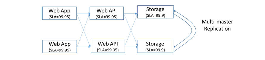
The implementation shown in Figure 3 can only be realized through multiple Azure regions because of the lack of control on the compute cluster and storage stamp selection in a single Azure region. The only reliable way of getting desired redundancy is to deploy the complete stack on each region as shown in Figure 4.
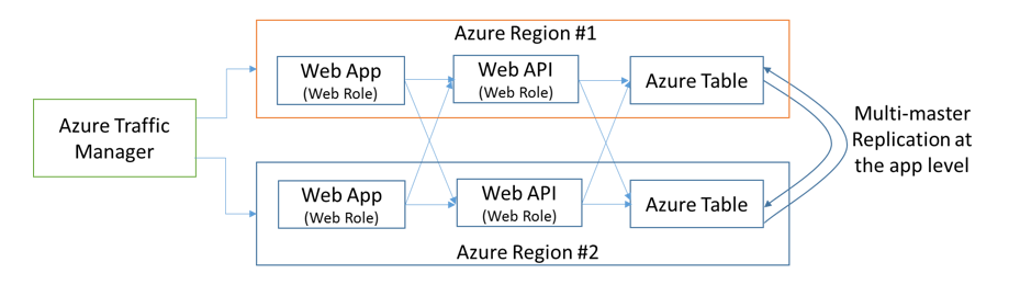
Figure 5: DMR architecture deployed to two Azure regions
Affinity-less interaction between application layers in an active-active deployment shown above is too complex to implement due to the near real time multi-master replication requirements of the persistent application state (e.g. Azure Table) resulting from the arbitrary cross DC access of the application layers. No matter which storage technology is used, changes to the business entities have to be written to storage tables in both the data centers. Preventing arbitrary layer interaction between data centers reduces the state complexity issues and hence the architecture can be simplified as shown below:
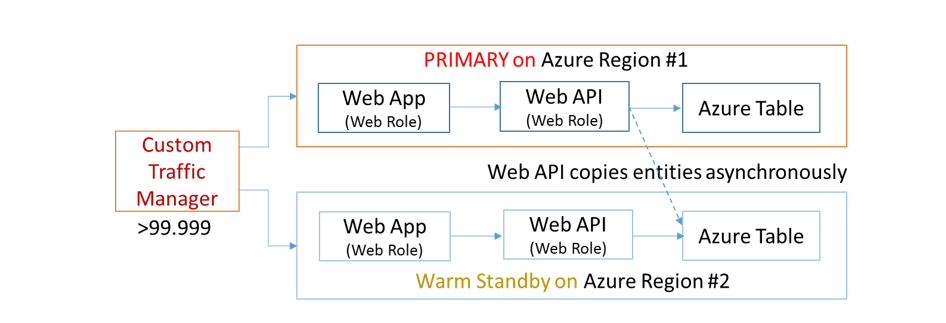
Figure 6: DMR architecture deployed to two Azure regions
Let us describe the changes that we made from the hypothetical system in Figure 5 to an implementable model.
The inter-layer communications between the data centers is removed due to the complexities involved with the multi-master write activities. Instead of an active-active model we selected an active-passive model where the secondary is in a warm standby mode.
Azure Traffic Manager is replaced with a custom traffic manager (e.g. an on-premise distributed traffic manager or a client rotating through a list of URLs) that can have higher availability than Azure Traffic Manager’s SLA of 99.99. With Azure Traffic Manager usage, the max reliability of even the multi-region deployment will mathematically be <= 99.99.
Since Azure Table doesn’t support multi-master replication and doesn’t give storage account level control to failover (entire stamp has to fail6) to the geo replicated secondary for writes, application level writes are required. In order for this to work, a separate storage account is required on the secondary data center.
Web API level Azure Table replication requires local writes to be asynchronously queued (e.g. storage or service bus queue) to the remote storage table because otherwise it will reduce the SLA due to the tight coupling of the remote queuing infrastructure.
The above implementation can turn into an active-active set up if the storage state can be cleanly partitioned across multiple deployments. The transactional data from such partitions can be asynchronously brought into a single data warehouse for analytics4.
Content driven applications like media streaming, e-Books, and other services can easily build systems with 99.999 on Azure by distributing content through multiple storage accounts located in multiple Azure regions. So, with shared nothing architecture the set up in Figure 3 can easily be translated into an active-active deployment.
Triple Modular Redundancy (TMR)
Triple modular redundancy, as the name indicates, involves the creation of 3 parallel execution paths for each component that is prone to fail. TMR can dramatically raise the reliability of the logical component even if the underlying physical component is highly unreliable. For most software systems, DMR is good enough unless the systems (such as industrial safety systems and airplane systems) can potentially endanger human life. In fact, Space Shuttle2 employed quadruple redundancy for its flight-control systems.

The Azure architecture shown in Figure 3 is morphed into the Figure 7 shown below for TMR:
Figure 7: TMR architecture deployed to three Azure regions
The theoretical availability for such a system is as shown below:
Rsystem = (1 – (1-0.998) x (1-0.998) x (1-0.998)) = 0.99999999
99.999999 is unthinkable for most cloud-hosted systems because it is an extremely complex and expensive undertaking. The same architecture patterns that are applied to DMR can easily be applied to TMR, so we will not rehash the strategies here.
CAP Theorem and High Availability of Azure Deployments
Distributed multi-region deployment is a key success factor for building highly available systems on cloud platforms including Microsoft Azure. Per CAP theorem8, you can only guarantee two of the three (C – Consistency, A- Availability, P – network Partition tolerance) systemic qualities in applications that use state machines. Given that multi-region deployments on Azure are already network partitioned, the CAP theorem can be reduced to the inverse relationship of C and A. Consequently it is extremely hard to build a highly consistent system that is also highly available in a distributed setting. Availability in CAP theorem refers to the availability of the node of a state machine, and in our case Azure Table is such a logical node. In this case, the overall deployment’s Availability and Consistency are correlated to A and C of Azure Table . Azure Table can be replaced with any state machine (e.g. Mongo DB, Azure SQL Database, and Cassandra) and the above arguments are still true.
High availability at the order of 99.99 and above requires the relaxation of system’s dependency on state consistency. Let us use a simple e-commerce scenario where shoppers can be mapped to their respective zip codes. We needed TMR due to the availability requirement of 99.999 or above for this hypothetical system. We can safely assume that the reference data like product catalog is consistently deployed to all the Azure regions.
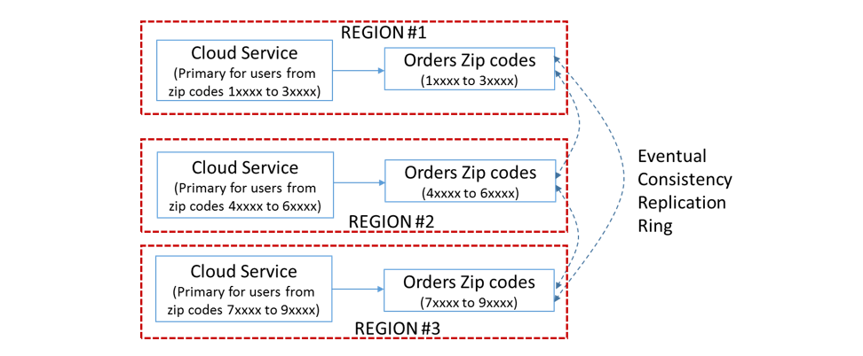
Figure Figure 8: Embarrassingly parallel data sets for high availability
This multi-region deployment requires the identification of embarrassingly parallel data sets within the application state and map each deployment as the primary for mutability of the respective data sets. In this case, the deployment in each region is mapped to a set of zip codes and all the transactional data from the users belonging to these zip codes will be written to the respective regional database partition (e.g. Azure Table). All the three regions are serving the same application in an active-active setting. Let us assume that the replication latency is 15 min for an entity write. We could set up the following mapping for primary and fail-over operations:
| Zip Code Range | Primary | Secondary | Tertiary |
|---|---|---|---|
| 10000 to 39999 | Region #1 | Region #2 | Region #3 |
| 40000 to 69999 | Region #2 | Region #3 | Region #1 |
| 70000 to 99999 | Region #3 | Region #1 | Region #2 |
If Region #1 is down, users can be sent to other regions with appropriate annotation that their shopping carts and order status are not current. Users can continue browsing the catalog, modify the shopping cart (albeit an older one) and view the delayed order status. Given that this only happens at the failure of a region, which is expected to be a rare event, users may be more forgiving than the dreaded “System is down and comeback later” message.
Tying this back to CAP theorem, we attained higher availability through an active-active TMR deployment at the expense of the overall consistency of the state data. If system functionality can’t tolerate data inconsistency resulting from the replication latency, one can’t use eventual consistency model. Strong consistency implementation between Azure regions can result in reduced availability due to the cascading effect of a region’s failure because of the tight coupling with other regions.
Summary
Given the current SLA model of Azure managed services such as compute, storage, networking and other supporting services, architecting systems with high availability like 99.99 and beyond requires a multi-region deployment strategy. In most cases the ceiling for a single region Azure deployment is 99.95 or below due to the compounding effect of the SLAs of multiple services used in a typical cloud service. Redundancy with shared nothing architecture is the key success factor of achieving high system reliability. Building highly reliable systems of 99.99 or above is an expensive undertaking that requires deliberate designs and architecture practices regardless of whether it is for the cloud or on-premise. Factoring in the trade-offs between consistency and availability into the application architecture will produce the desired solution outcome whose complexity can be manageable.
Thanks to Mark Russinovich, Patrick Chanezon, and Brent Stineman for helping me in improving this article.
References
- "Redundant System Basic Concepts." - National Instruments. N.p., 11 Jan. 2008. Web. 30 Mar. 2014. https://www.ni.com/white-paper/6874/en/.
- "Computers in the Space Shuttle Avionics System." Computer Synchronization and Redundancy Management. NASA, n.d. Web. 30 Mar. 2014. https://www.hq.nasa.gov/office/pao/History/computers/Ch4-4.html.
- Russinovich, Mark. "Windows Azure Internals." Microsoft MSDN Channel 9. Microsoft, 1 Nov. 2012. Web. 30 Mar. 2014. https://channel9.msdn.com/Events/Build/2012/3-058.
- McKeown, Michael, Hanu Kommalapati, and Jason Roth. "Disaster Recovery and High Availability for Windows Azure Applications." Msdn.microsoft.com. N.p., n.d. Web. 30 Mar. 2014. https://msdn.microsoft.com/en-us/library/windowsazure/dn251004.aspx.
- Mercuri, Marc, Ulrich Homann, and Andrew Townsend. "Failsafe: Guidance for Resilient Cloud Architectures." Msdn.microsoft.com. Microsoft, Nov. 2012. Web. 30 Mar. 2014. https://msdn.microsoft.com/en-us/library/jj853352.aspx.
- Haridas, Jai, and Brad Calder. "Windows Azure Storage Redundancy Options and Read Access Geo Redundant Storage." Microsoft MSDN. Microsoft, 11 Dec. 2013. Web. 30 Mar. 2014. https://blogs.msdn.com/b/windowsazurestorage/archive/2013/12/04/introducing-read-access-geo-replicated-storage-ra-grs-for-windows-azure-storage.aspx.