Introduction
While fuzzing, you may need to extrapolate or describe analytically a “fuzzing curve”, which is the dependency between the number of bugs found and the count of fuzzing inputs. Here I will share my approach to deriving an analytical expression for that curve. The results could be applied for bug flow forecasting, return-on-investment (ROI) analysis, and general theoretical understanding of some aspects of fuzzing.
If you are wondering about things like “what is fuzzing?” here is a little FAQ:
Q: So, what is fuzzing?
Microsoft Research Podcast

AI Frontiers: AI for health and the future of research with Peter Lee
Peter Lee, head of Microsoft Research, and Ashley Llorens, AI scientist and engineer, discuss the future of AI research and the potential for GPT-4 as a medical copilot.
A: “Fuzz testing or fuzzing is a software testing technique <…> that involves providing invalid, unexpected, or random data to the inputs of a computer program. The program is then monitored for exceptions such as crashes, or failing built-in code assertions or for finding potential memory leaks. Fuzzing is commonly used to test for security problems in software or computer systems.” (Wikipedia Wikipedia definition)
Basically, every time you throw intentionally corrupted or random input at the parser and hope it will crash, you do fuzzing.
Q: What is a fuzzing curve?
A: That is simply the dependency between the number of unique bugs (e.g., crashes) found and the number of inputs provided to the program, also called “iterations”. A fuzzing curve, being a special case of a bug discovery curve, may look like this:
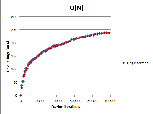
[For the record, the data is simulated and no real products have suffered while making this chart.]
Q: Why do we need to know fuzzing curve equation?
A: If you don’t know the true equation of it, you can’t justifiably extrapolate it. If a choice of extrapolation function is random, so is the extrapolation result, as the picture below illustrates:
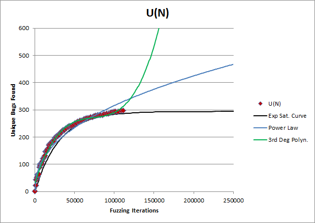
Imagine you tell your VP that you need to continue fuzzing and budget $2M for that. They may reasonably ask “why?” At that point, you need a better answer than “because we assumed it was a power law”, right?
Q: Has there been any past research of this area?
A: Plenty, although I haven’t seen yet a fuzzing curve equation published. To mention a couple of examples:
-
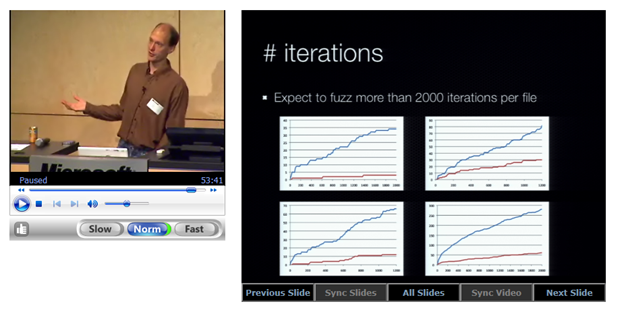
- In 2008, Jason Shirk, Lars Opstad, and Dave Weinstein presented their Fuzzed enough? When it’s OK to put the shears down work at Blue Hat 2008. They conducted analysis of fuzzing results for 250+ Windows Vista parsers and found empirically that 500,000 iterations appeared to be enough to detect at least one crash in most crashing parsers. They also ran one of the fuzzers for 27 million iterations but were unable to “flatten out” the fuzzing curve.
- Charlie Miller’s Fuzzing “truths” discovered while fuzzing 4 products with 5 lines of Python from BlueHat 2010 is closely related to the topic of this blog post. In that work, the results of “dumb” fuzzing against four different parsers are discussed. Classic pictures of fuzzing curves are presented and a notion of their saturation is introduced. The approach to fuzzing ROI assessment was in lines of “when the curve flattens out, you know you’d fuzzed enough”. The lack of theoretical ground for such prediction is explicitly called out: “I don’t know how long the fuzzing needs to continue… it would be awesome to know how many iterations are required to flatten out each of these curves”
Q: Can this work replace any of the following:
-
- Targeted or systematic/deterministic fuzzing?
- Analysis of additional fuzzing data such as stack traces proximity or code coverage?
A: No.
Q: Can it provide any of the following:
-
- Prediction of the total number of bugs in a product discoverable by any combination of fuzzers?
- A method to point out specific bugs or areas of higher bug density in the product (as opposed to only counting bugs)?
- Information on new or existing zero-day vulnerabilities?
A: No.
If you are still interested – let’s continue after the Standard Disclaimer:
Information and opinions expressed in this post do not necessarily reflect those of my employer (Microsoft). My recommendations in no way imply that Microsoft officially recommends doing the same. Any phrases where it may look as if I don’t care about customer’s security or recommend practices that increase the risk should be treated as purely accidental failures of expression. No figures or statements given here imply any conclusions about the actual state of security of Microsoft’s or any other products. The intent of this text is to share knowledge that aims to improve security of software products in the face of limited time and resources allocated for development. The emotional content represents my personal ways of writing rather than any part of the emotional atmosphere within the company. While I did my best to verify the correctness of my calculations, they may still contain errors, so I assume no responsibility for using (or not using) them.
Derivation of the equation
The following conditions, further referred to as “static fuzzing”, are assumed:
- The product does not change during fuzzing.
- The fuzzer does not experience major configuration changes during fuzzing.
- There are no super-crashers in the product. Those are bugs that manifest with probability sufficiently close to 1 (e.g., over 10%). A product with super-crashers in it is likely so unstable that it won’t be ready for fuzz testing anyways.
- The definitions of bugs uniqueness or exploitability do not change throughout fuzzing.
- Fuzzing is random or nearly random in a sense that bug discovery chances do not depend on past results, or such dependency extends only over bug sets much smaller than the total number of bugs found.
Let’s start with a hypothetical product with B bugs in it where each bug has exactly the same fixed probability p > 0 of being discovered upon one fuzzing iteration.
Actually, the “bug” does not have to be a crash, and “fuzzing iteration” does not have to apply exactly against a parser. A random URLs mutator looking for XSS bugs would be described by the same math.
Consider one of these bugs. If the probability to discover it in one iteration is p, then the probability of not discovering it is 1 – p.
What are the chances that this bug will not be discovered after N iterations, then? In static fuzzing, each non-discovery is an independent event for that bug, and therefore the answer is:
![]()
Then, the chance that it will be eventually discovered after N iterations is:
![]()
Provided there are B bugs in the product, each one having the same discovery probability P(N), the mathematical expectation of the number of unique bugs U found by the iteration number N is:
![]()
If all bugs in the product had the same discovery probability that would’ve been the answer. However, real bugs differ by their “reachability” and therefore by the chance of being found. Let’s account for that.
Consider a product with two bug populations, B1 and B2, with discovery probabilities of p1 and p2 respectively. For each population, the same reasoning as in (10)-(30) applies, and (30) changes to:
![]()
Extending that logic onto an arbitrary number Q of populations {Bq} one arrives at:
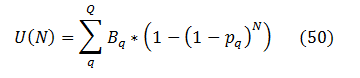
(q enumerates bug populations here)
Let’s introduce bugs distribution function over discovery probability G(p) per definition:
Bq(p) = G(pq)*dp
Then (50) is replaced by integration:
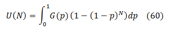
Let’s recall that (1 ‑ p)N = eN*Ln(1 ‑ p). In the absence of super-crashers G(p) is significant only at very small probabilities p << 1. Thus, the logarithm could be expanded into first order series as Ln(1‑p) ≈ ‑p, and then:
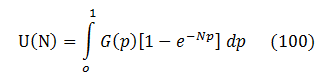
This is the generic analytical expression for a static fuzzing curve.
Can it be simplified further? I believe the answer is “no”, and here is why.
Let’s look at the first derivative of U(N) which is easy to obtain from (100):
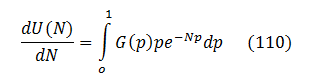
Since G(p) is a distribution function, it is non-negative, as well as the exponent and p. Therefore,
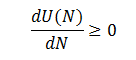
for any N.
Similarly, the 2nd derivative could be analyzed to discover that it is strictly non-positive:
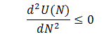
Repeating the differentiation, it is easy to show that
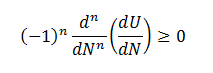
for any n>=0.
That is a very prominent property. It is called a total (or complete) monotonicity and only few functions possess it. Sergei Bernstein has shown in 1928 [see Wikipedia summary] that any function that is totally monotonic must be a mixture of exponential functions and its most general representation is:
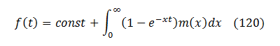
where m(x) is non-negative.
In our case the first derivative of U(N) is totally monotonic. Therefore, U(N) with possible addition of some linear terms like a + b*N belongs to the same class of functions. Therefore, (100) is already a natural representation for U(N) and there is no simpler one. Any attempt to represent U(N) in an alternative non-identical way (e.g., via a finite polynomial) would destroy the complete monotonicity of U(N), and that would inevitably surface as errors or peculiarities in further operations with U(N).
So let’s settle upon (100) as the equation of a static fuzzing curve.
G(p)?
But wait! Expression (100) depends on the unknown function G(p). So it’s not really the answer. It just defines one unknown thing through another. How is that supposed to help?
In a sense, that’s true. The long and official response to that is this: you start fuzzing, observe the initial part of your fuzzing curve, solve the inverse problem to restore G(p) from it, plug it back to (100) and arrive to the analytical expression of your specific curve.
But here is a little shortcut that can make things easier.
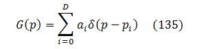
Every function could be represented (at least for integration purposes) as a collection of Dirac delta-functions, so let’s do that with G(p):
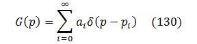
where ai>0 and pi>0 are some fixed parameters.
Most of the time, only small ranges of probabilities contribute significantly to fuzzing results. That’s because “easy” bugs are already weeded out, and “tough” ones are mostly unreachable. To reflect that, let’s replace the infinite sum with a fixed small degree D corresponding to the most impactful probability ranges:
Substituting that into (100) results in the following fuzzing curve equation:
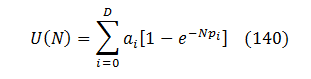
After some experiments I found that D = 1 already fits and extrapolates real fuzzing curves reasonably well, while D = 3 produces a virtually perfect — fit at least on the data available to me.
Finally, at the very early fuzzing stages (140) could be reduced even further to:
![]()