"Cartographic Adjustment" of Spatial Data for SQL Server Reporting Services, Part 4
In the previous posts I indicated that this would be the last post in this series but it turned out that I was a bit optimistic. In order to make the final Report Builder post relevant, some interesting data for analysis was needed. In this post we describe where to find and how to load State-based population data - our "interesting data".
- Locate data source and download (Part 1)
- Load the data into SQL Server (Part 1)
- Remove unwanted features, simplify Alaska and Hawaii spatial features (Part 2)
- "Reposition" Alaska and Hawaii cartographically (Part 3)
- Locate and load State-based population data
- Use the data in the new SQL Server Report Builder
LOCATING STATE POPULATION DATA
Our search for population data by State was satisfied at the US Census Bureau Population Estimates site. There are a number of data files which are available, but I chose Population, Population change and estimated components of population change: April 1, 2000 to July 1, 2008 (NST-EST2008-alldata).
This data is delivered as commas-separated-value (CSV) ASCII. This data was opened in Excel and saved as Text (Tab delimited).
LOADING STATE POPULATION DATA
Now we are going to use FME to do something for which it is not well known - loading data with no spatial component.
ADDING THE STATE POPULATION DATA AS THE SOURCE DATASET
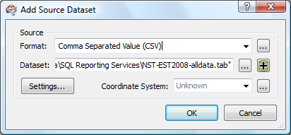
In FME-speak, all ASCII data is format "Comma Separated Value (CSV)". Consequently, we choose CSV as our format - never mind that our data is tab separated values. Next we locate the data using the "..." menu button. After both the Format: and the Dataset: text fields are populated, choose the "Settings..." button.
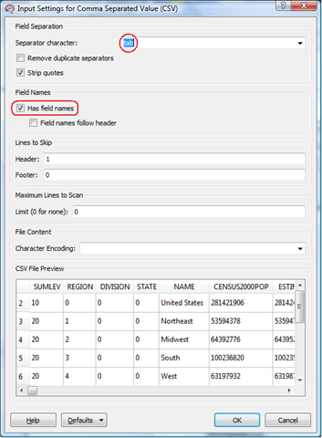
The "Settings..." button brings up a new menu panel which allows us to correctly define our field separator as "tab". Since our ASCII file contains field names, we want to make sure that this record is not interpreted as data. In fact, we will use the field names as the columns names in the final database table. The CSV File Preview provides visual verification that we are correctly interpreting the file structure.
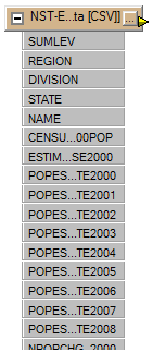
The source data now appears on the workbench canvas:
ADDING THE DESTINATION DATASET
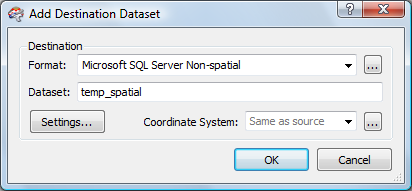
The destination dataset will be our new database table which we will name us_states_population. Here is the first menu panel that appears when we add a new Destination Dataset:
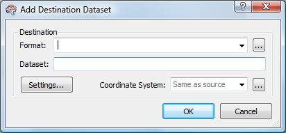
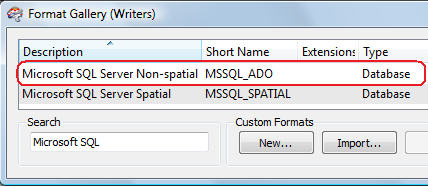
Our first task is to choose the correct output format. We have two potential choices for SQL Server. In this case, since the new database table will not have a spatial column, we want the Microsoft SQL Server Non-spatial (MSSQL_ADO) format:
Note: If we chose the Microsoft SQL Server Spatial (MSSQL_SPATIAL) format, the data load would work correctly but would have a spatial column defined in the output table, populated with NULL values.
Next, we want to select the "Settings..." button. This allows us to define our server instance, dataset and authentication. The use of the term "Dataset" is a bit confusing for database users. What FME is asking for, in this case, is the database name (in our case, temp_spatial):
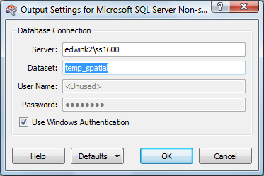
With the destination defined, hit "OK" to continue...
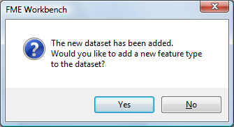
FME next asks if you would like to add a new feature type to the dataset. This can be interpreted as "Would you like to add a new table to the database?", so we need to answer Yes:
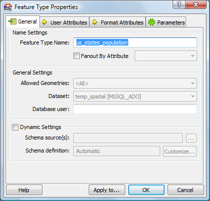
The Feature Type Properties (a.k.a. Table Properties) panel asks for the Feature Type Name. We supply the name of the database table to hold the population data: us_states_population
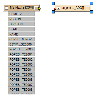
We hit OK at this point and the destination end point appears on the workbench canvas:
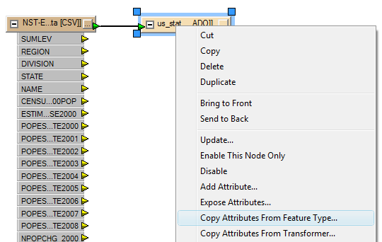
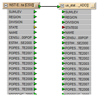
Next, we connect the source and the destination and the upper connection triangles turn green, indicating success. Now, right click on the destination data and choose "Copy Attributes From Feature Type...":
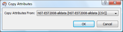
The Copy Attributes menu panel will now display. Choose, "Copy Attributes From:" the only option will be the correction option, in this case:
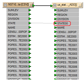
The workbench canvas now appears as follows. It is unclear why FME choose to rename the STATE column but it did (to STATE00). This causes the implicit connections between source and destination columns to be undefined (yellow connection triangle on source and red connection triangle on the destination).
To associate the STATE (source) and STATE00 (destination) columns, drag a line between the two:
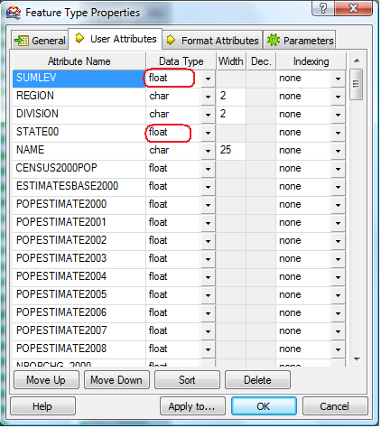
The final task is to check the data types and definitions associated with each column. Here are the original definitions:
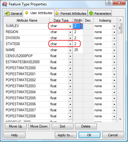
The SUMLEV and STATE00 columns are both defined as float. While we are not interested in the SUMLEV column, the STATE00 column needs to be defined as char 2 for compatibility with the STATEFP column in the us_states table, to which we will join this table later on:
LOAD THE STATES POPULATION DATA
Execute the FME workspace to load the data into a SQL Server table, us_states_population. The last step is to rename the STATE00 to STATE in Management Studio.
We are now ready to create our first map report in the Report Builder. This will be described in Part 5.
Technorati Tags: Non-spatial,data,population,Census,loading,Safe Software,FME 2010 Beta,FME,Feature Manipulation Engine,SQL Server,2008,non-spatial