Statistics on system tables and query performance

Recently I was helping a customer design a database with a very large number of database objects – hundreds of schemas, a few thousands of stored procedures, hundreds of partitioned tables, with most tables containing between two hundred and a thousand partitions. Once all these objects were created, I had to write a catalog metadata query that went something like this: “Find the partition of a table in schema A that has the largest number of pages of all partitions in that table, with the limitation that the table must have more than one partition and may not be referenced by a foreign key constraint, and has a view in schema B with the same name.” (As little sense as this probably makes, there was a perfectly good reason why this query was needed.)

With the plethora of catalog views and DMVs in SQL Server, writing this query wasn’t particularly hard. In this case, it involved sys.schemas, sys.tables, sys.views, sys.partitions, sys.indexes, sys.dm_db_partition_stats, and sys.data_spaces. However, while the query returned correct results, its performance was very poor: it took about twenty seconds to return the row I was after. Looking at the query plan, I noticed something that would normally be a direct clue to the cause of poor performance: while the actual number of rows passing through various iterators in the plan varied, the estimated number of rows was always 1. In other words, the estimates used by the optimizer were inaccurate, resulting in suboptimal plan and poor performance.

If the query used regular user tables, the next troubleshooting step would be to update statistics on these tables in the hopes of giving the optimizer better estimates. But in this case, the query used only catalog views and DMVs, and on first glance, there was no statistics in sight. However, looking at the query plan, I saw that the objects referenced in the iterators were actually hidden system tables, i.e. sys.sysclsobjs, sys.sysidxstats, sys.sysschobjs, sys.syssingleobjrefs, etc. While it is not possible to query these tables directly (unless using the DAC connection), their definition can still be viewed with the sp_help stored procedure. The result from sp_help includes the indexes defined on these tables, and for each index, corresponding statistics can also be viewed with DBCC SHOW_STATISTICS.

When I did that, the reason for inaccurate estimates was clear – even though most tables had a rather large number of rows corresponding to the multitude of objects in the database, in many cases the statistics were dated prior to the time when database objects were created, and showed completely inaccurate density and distribution. Once I ran UPDATE STATISTICS on each index of the system tables, the query returned in less than a second.

© 2019 Microsoft. All rights reserved.

Estimating data compression savings for entire database

The sp_estimate_data_compression_savings system stored procedure in SQL Server 2008 estimates how much space can be saved by compressing a single partition of an index on a table. Performing this estimation for many tables, indexes, and partitions manually is a tedious task.

The attached script is a wrapper for the sp_estimate_data_compression_savings procedure, that calls it on each partition in the database and in the end outputs a single result set. This multi-row result set is similar to the one-row set from sp_estimate_data_compression_savings. It contains three rows for every partition in the database, one row for each available compression option (NONE, ROW, PAGE). The three totals rows, presenting average compression estimates for the entire database, are at the top of the result set. As written, the script includes only the database level totals, however it is not hard to add other levels of aggregation (i.e., by schema, table, index, or a combination thereof), by modifying the GROUPING SETS clause in the last SELECT statement.

Please note that for large databases, the script can take a long time to complete. To gauge progress, the script outputs status messages referencing the object, index, and partition used as arguments for the current call to sp_estimate_data_compression_savings.

The sp_estimate_data_compression_savings stored procedure is available only in the Enterprise, Developer, or Datacenter editions of SQL Server 2008 and SQL Server 2008 R2.

EstimateCompressionSavings.sql

© 2019 Microsoft. All rights reserved.

Point-in-time restore and knowing where to stop


In some disaster recovery scenarios, a database needs to be restored to a point in time before a particular operation has occurred, e.g. before a user mistakenly dropped a table, ran a DELETE or UPDATE with no WHERE clause, etc. If the database is in the full recovery mode and the log backup chain is not broken, then this is can be achieved by using the RESTORE LOG command with the STOPAT clause. The STOPAT clause is used to specify a point in time when the recovery should stop during log restore. In this case, this would be the time immediately before the transaction containing the erroneous DROP TABLE command is committed. The problem is, frequently you do not know the specific point in time when the user made the mistake. On one hand, to minimize data loss, you need to stop the recovery immediately before the transaction commit. On the other hand, if you overshoot that point in time when restoring the log, you need to start the restore sequence from scratch, restoring the latest full backup, differential backups (if any), and a set of transaction log backups. This may have to be repeated several times, until you arrive at the exact STOPAT time by trial and error. Needless to say, this approach may not be realistic, particularly for large databases.

Luckily, in many cases there is a way to determine the precise point where the restore should stop. This approach may be difficult to implement in some cases, particularly on systems with a lot of write activity, but when it does work, it can save you a lot of time during disaster recovery, while minimizing data loss.

I am going to assume that the transaction log containing the transaction with the user error operation has been backed up – if that is not the case, you will need to perform the tail-log backup before starting with the steps below.

The approach is to use the undocumented fn_dump_dblog() table-valued function, which provides a rowset over the contents of a transaction log backup file (I described the function in an earlier blog post). Each row in the function’s result set represents a log record in the log backup file specified as the function argument. The first column in the result set is named Current LSN, and represents the Log Sequence Number of each log record in the backup file. The RESTORE LOG command has the STOPBEFOREMARK clause, which similarly to the STOPAT clause allows the recovery to be stopped immediately before a particular LSN (in SQL Server 2005 and later). Therefore, if we can determine the LSN associated with the commit of the transaction that included the erroneous command, we can specify that value in the STOPBEFOREMARK clause, and thus restore the database to a point in time immediately before the disaster occurred. The difficulty here is that it may not be easy or even possible to find the erroneous command in the large result set returned by the fn_dump_dblog() function, particularly if the database had a lot of write activity when the erroneous command was run.

The sample script below demonstrates the approach.

-- Create test database, switch it to full recovery model

CREATE DATABASE PointInTimeRestore;
GO

USE PointInTimeRestore;
GO

ALTER DATABASE PointInTimeRestore SET RECOVERY FULL;
GO

— Create the initial full backup
BACKUP DATABASE PointInTimeRestore
TO DISK = ‘C:\MSSQLData\MSSQL10.SS2008\MSSQL\Backup\PointInTimeRestore.bak’;
GO

— Create test table, insert sample data

CREATE TABLE Table1
(
Col1 INT PRIMARY KEY
);
GO

INSERT INTO Table1 (Col1)
VALUES (1), (2), (3);
GO

— Simulate user error and drop the table
DROP TABLE Table1;
GO

— Backup the log containing the erroneous command
BACKUP LOG PointInTimeRestore
TO DISK = ‘C:\MSSQLData\MSSQL10.SS2008\MSSQL\Backup\PointInTimeRestore.trn’;
GO

— Change database context to allow restore of the test database
USE tempdb;
GO

— Restore the database, but do not run recovery to be able to restore transaction logs
RESTORE DATABASE PointInTimeRestore
FROM DISK = ‘C:\MSSQLData\MSSQL10.SS2008\MSSQL\Backup\PointInTimeRestore.bak’
WITH REPLACE, NORECOVERY;
GO

— Examine log backup contents to find the LSN corresponding to the DROP TABLE transaction
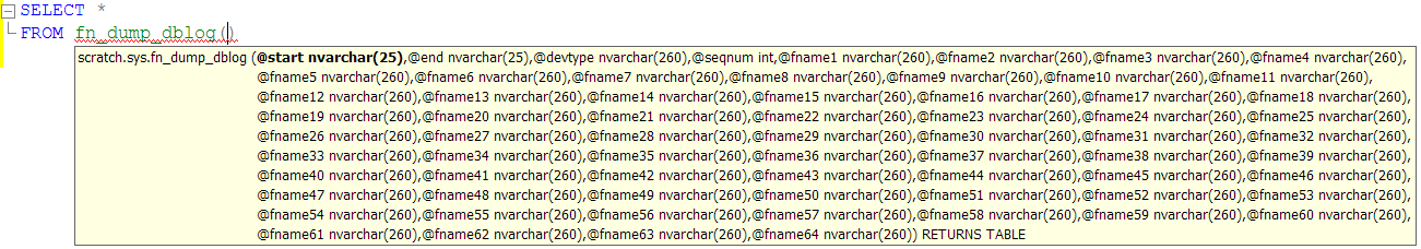
SELECT *
FROM fn_dump_dblog
(
DEFAULT, DEFAULT, DEFAULT, DEFAULT,
‘C:\MSSQLData\MSSQL10.SS2008\MSSQL\Backup\PointInTimeRestore.trn’,
DEFAULT, DEFAULT, DEFAULT, DEFAULT, DEFAULT, DEFAULT, DEFAULT, DEFAULT, DEFAULT,
DEFAULT, DEFAULT, DEFAULT, DEFAULT, DEFAULT, DEFAULT, DEFAULT, DEFAULT, DEFAULT
);
GO

/*
In this case, the log record corresponding to the commit of the transaction
that dropped the Table1 table can be easily found in the result set – the
Operation column for the row is LOP_COMMIT_XACT, and the value in the
Transaction ID column corresponds to the value in the Transaction ID column for
an earlier row with Operation LOP_BEGIN_XACT and Transaction Name DROPOBJ.
We also happen to know that this is the only table that was dropped at the time
in the End Time column.
The LSN in the Current LSN column is 0000002a:00000074:0036.
*/

/*
Restore log to the point in time just before the table was dropped.
Note that we need to prepend 0x to the LSN value –
will get the “The named mark does not identify a valid LSN” an error otherwise.
*/
RESTORE LOG PointInTimeRestore
FROM DISK = ‘C:\MSSQLData\MSSQL10.SS2008\MSSQL\Backup\PointInTimeRestore.trn’
WITH STOPBEFOREMARK = ‘lsn:0x0000002a:00000074:0036’;
GO

— Confirm that the table is again present in the database
USE PointInTimeRestore;
GO

SELECT *
FROM Table1;

© 2019 Microsoft. All rights reserved.

Adding the IDENTITY property to a column of an existing table


Until SQL Server 2005, it was not possible to alter a column in an existing table to add the IDENTITY property. To achieve that, it was necessary to create a new table with an IDENTITY column, and move the data into that table. For large tables, this could be problematic.

With the introduction of table partitioning in SQL Server 2005, there is a neat solution to this problem. As described in Transferring Data Efficiently by Using Partition Switching, the schemas of the source and destination tables in the ALTER TABLE … SWITCH statement have to match exactly (loosely speaking – the specific requirements are quite detailed). However, and that’s the key part here, the topic says that “The IDENTITY property is not considered.” In other words, the target table can have the IDENTITY property on a column, even though the source table does not have it. Therefore, we can switch the data from the source table into the target table, which is a very fast metadata-only operation, and gain the IDENTITY property without having to physically move data from one table to another. The target table and associated constraints can then be renamed to match the original source table.

Here’s a script that demonstrates this approach:

/*
A table without an IDENTITY column.
We want to add the IDENTITY property to the Col1 column
*/
CREATE TABLE AddIdentity (
Col1 INT NOT NULL,
Col2 VARCHAR(10) NOT NULL,
CONSTRAINT pkAddIdentity PRIMARY KEY (Col1)
);

/*
A temporary table, with the schema identical to the AddIdentity table,
except that the Col1 column has the IDENTITY property
*/
CREATE TABLE AddIdentityTemp (
Col1 INT NOT NULL IDENTITY(1,1),
Col2 VARCHAR(10) NOT NULL,
CONSTRAINT pkAddIdentityTemp PRIMARY KEY (Col1)
);

— Insert test data
INSERT INTO AddIdentity (Col1Col2)
VALUES (1‘a’);

— Switch data into temporary table
ALTER TABLE AddIdentity SWITCH TO AddIdentityTemp;

— Look at the switched data
SELECT Col1Col2
FROM AddIdentityTemp;

— Drop the original table, which is now empty
DROP TABLE AddIdentity;

— Rename the temporary table, and all constraints, to match the original table
EXEC sp_rename ‘AddIdentityTemp’‘AddIdentity’‘OBJECT’;
EXEC sp_rename ‘pkAddIdentityTemp’‘pkAddIdentity’‘OBJECT’;

— Reseed the IDENTITY property to match the maximum value in Col1
DBCC CHECKIDENT (AddIdentityRESEED);

— Insert test data
INSERT INTO AddIdentity (Col2)
VALUES (‘b’);

— Confirm that a new IDENTITY value has been generated
SELECT Col1Col2
FROM AddIdentity;

© 2019 Microsoft. All rights reserved.

Tempdb configuration check script


There is a number of well known best practices for configuring the tempdb database on SQL Server. Specifically:

  • Multiple data files are used (some sources recommend 1 data file per CPU core, while others recommend anywhere from 1/4 to 1 file per CPU core)
  • All data files have equal size
  • All data files have equal maximum size
  • All data files have equal growth increment
  • No data files have percent growth increment

Note that the multiple data file recommendation is usually presented in terms of the number of files per CPU core. So how do we determine the number of CPU cores to use in this calculation? In the general case, it would be incorrect to use the total number of cores in the machine, because not every core may be in use by SQL Server due to a non-default CPU affinity mask. Ultimately, what matters here is not so much the number of cores, but the number of scheduler threads. The reasoning behind this best practice is to provide a separate data file for each scheduler thread, so that multiple simultaneous tempdb space allocation requests can use separate data files, thus reducing space allocation contention.

Starting from SQL Server 2005, the number of schedulers for a SQL Server instance can be easily found from the scheduler_count column in sys.dm_os_sys_info DMV. This is the value used in the query below to determine if the multiple data file recommendation is followed. The specific rule I’m using here is between 1/2 and 1 data file per scheduler. If needed, it is trivial to change the query for a different definition of this best practice.

Here is a query that returns a single row result set showing if tempdb is configured according to these best practices. This can be run against multiple instances using a multi-server query in SSMS 2008, to quickly find out if tempdb is configured according to best practices across the enterprise.

WITH
TempdbDataFile AS
(
SELECT  size,
max_size,
growth,
is_percent_growth,
AVG(CAST(size AS decimal(18,4))) OVER() AS AvgSize,
AVG(CAST(max_size AS decimal(18,4))) OVER() AS AvgMaxSize,
AVG(CAST(growth AS decimal(18,4))) OVER() AS AvgGrowth
FROM tempdb.sys.database_files
WHERE   type_desc 'ROWS'
AND
state_desc 'ONLINE'
)
SELECT  CASE WHEN (SELECT scheduler_count FROM sys.dm_os_sys_info)
BETWEEN 
COUNT(1)
AND 
COUNT(1) * 2
THEN 'YES'
ELSE 'NO'
END
AS 
MultipleDataFiles,
CASE SUM(CASE size WHEN AvgSize THEN ELSE END)
WHEN COUNT(1THEN 'YES'
ELSE 'NO'
END AS EqualSize,
CASE SUM(CASE max_size WHEN AvgMaxSize THEN ELSE END)
WHEN COUNT(1THEN 'YES'
ELSE 'NO'
END AS EqualMaxSize,
CASE SUM(CASE growth WHEN AvgGrowth THEN ELSE END)
WHEN COUNT(1THEN 'YES'
ELSE 'NO'
END AS EqualGrowth,
CASE SUM(CAST(is_percent_growth AS smallint))
WHEN THEN 'YES'
ELSE 'NO'
END AS NoFilesWithPercentGrowth
FROM TempdbDataFile;

© 2019 Microsoft. All rights reserved.

Query performance, scalar UDFs, and predicate pushdown


Recently I had to troubleshoot a query that performed much slower than expected. The solution to that seemed sufficiently interesting to warrant a write-up, and the root cause of the problem reinforced a well-known best practice of avoiding scalar user-defined functions in set-based queries.

The original query looked like this:

SELECT  'Literal1',
u.Col2
FROM dbo.Table1 AS u
INNER JOIN dbo.Table2 AS l
ON u.Col2 l.Col2
WHERE   l.Col3 'Literal2'
AND
NOT EXISTS  (
SELECT  1
FROM dbo.Table2 AS l2
WHERE   u.Col2 l2.Col2
AND
Col3 'Literal1'
)
AND
dbo.UDF1(u.Col1) IS NOT NULL;

Table1 had about 3 million rows, and Table2 had about 7 million rows. In its original form, the query was running for more than one hour, while the requirement was that it would complete within minutes.

The scalar user-defined function (UDF) in the WHERE clause immediately stood out as a warning sign (highlighted). Using scalar UDFs in set-based queries is generally not recommended for two reasons:

  1. The function is invoked for each row in the set, and each invocation has a fixed and not insignificant cost, which is in addition to the cost of the statements in the function body.

  2. The optimizer cannot accurately estimate the cost of the function (which could vary greatly), therefore it may come up with less than optimal query plans.

For the query above, removing the UDF from the WHERE clause brought down the execution time to 12 seconds. Looking at the query plan, it was clear why it took so long to execute the original statement – a full clustered index scan of Table1 (all 3 million rows of it) was followed by a filter operator, where the UDF was applied to the Col1 column of Table1. In other words, rather than first reduce the set via joins with Table2 and then apply the UDF to that much smaller set, the optimizer chose to first filter millions of rows with the UDF. This is a fairly typical example of a sub-optimal plan caused by an inaccurate estimate (reason #2 above), which was in turn caused by the usage of an “opaque” scalar UDF.

The obvious workaround for this problem would be to remove the UDF-based filter from the WHERE clause, insert the resulting intermediate result set into a temporary table, and then select from that temporary table, filtering the much smaller intermediate result set with the UDF. However, I wanted to avoid a procedural approach, which would be more complex and less robust than a single set-based statement.

The first attempt to come up with a single statement that avoids the original problem looked like this:

SELECT  'Literal1',
up.Col2
FROM    (
SELECT  u.Col1,
u.Col2
FROM dbo.Table1 AS u
INNER JOIN dbo.Table2 AS l
ON u.Col2 l.Col2
WHERE   l.Col3 'Literal2'
AND
NOT EXISTS  (
SELECT 1
FROM dbo.Table2 AS l2
WHERE   u.Col2 l2.Col2
AND
l2.Col3 'Literal1'
)
AS up
WHERE dbo.UDF1(up.Col1IS NOT NULL;

Here we have a subquery in the FROM clause, and apply the filter with the UDF “on top” of the subquery, in the WHERE clause of the outer query. The intent is to evaluate the subquery first, before applying the filter. Unfortunately, this does not work – this query is logically equivalent to the original query, and SQL Server is at liberty to evaluate the predicates in the order that it deems optimal, which in this case still means filtering millions of rows in Table1 with the UDF-based filter, before joining with Table2.

Here is the query that did work (changes to previous attempt are highlighted):

SELECT  'Literal1',
up.Col2
FROM    (
SELECT  u.Col1,
u.Col2
FROM dbo.Table1 AS u
INNER JOIN dbo.Table2 AS l
ON u.Col2 l.Col2
WHERE   l.Col3 'Literal2'
AND
NOT EXISTS  (
SELECT 1
FROM dbo.Table2 AS l2
WHERE   u.Col2 l2.Col2
AND
l2.Col3 'Literal1'
)
AS up
CROSS JOIN  (
SELECT '' AS EmptyString
AS e
WHERE dbo.UDF1(up.Col1 e.EmptyStringIS NOT NULL;

The reason this succeeds in forcing the optimizer to evaluate the UDF filter after reducing the row set via joins is because we pass an expression, rather than a base column, to the function. The passed expression in this case is logically equivalent to the base column, but because it contains a reference to a column from a seemingly pointless outer query, the optimizer cannot push down the UDF-based filter to the inner subquery. In the plan generated for this query, the UDF executes only against a few hundred rows produced by the inner subquery, and the statement completes in 30 seconds – well within required time. Note that it wouldn’t be sufficient to use a literal empty string as the second part of the expression – to avoid predicate pushdown, it has to be a column from an outer query.

As a conclusion, this could be a useful query tuning technique for the specific case when the optimizer pushes down a filtering predicate (not necessarily UDF-based), and the resulting plan is less optimal than the one where the filter is evaluated later in the plan.

© 2019 Microsoft. All rights reserved.

Reading database transaction log with fn_dump_dblog()

While the format of SQL Server transaction log is not publicly documented, there is a number of ways to view the contents of the log. This is sometimes necessary for troubleshooting and forensic purposes. One way is the DBCC LOG command. Another is fn_dblog() table-valued function. Both are undocumented, however you can easily find unofficial documentation on various web sites and blogs.

If you use Intellisense in SSMS 2008, you may notice another function, called fn_dump_dblog():

This function provides the same rowset as fn_dblog(), but has some interesting functionality that makes it useful is some troubleshooting and recovery scenarios. Specifically, it can read not only transaction log of the current database, but also transaction log backups on either disk or tape.

The first two parameters, @start and @end, can be used to filter the output by a range of LSN values (you need to make sure that the LSN values start with ‘0x’). This is similar to fn_dblog(). If you use default values for all other parameters, the fn_dump_dblog() function behaves just like fn_dblog(), returning a rowset over the log of the current database.

The third parameter, @devtype, is where the differences between fn_dump_dblog() and fn_dblog() start. This parameter determines the type of backup device. You can specify either ‘DISK’ or ‘TAPE’. ‘DISK’ is the default.

The fourth parameter, @seqnum, is an integer that can be used to specify a particular backup within a backup device, when the same device has been used for multiple backups. Most backup devices contain only one backup, so usually this will be 1.

The fifth parameter is the fully-qualified path to the backup file on disk, when backup device type is ‘DISK’. Note that Intellisense displays this parameter simply as @fname1. Note that the SQL Server service account will need read permission on the backup file.

The sixth parameter, displayed as @fname2, can be used to provide the name of a backup file in the default backup directory for the SQL Server instance.

All other parameters appear to be unused (please post a comment if you find otherwise). Update 2012-05-18: Paul Randal just blogged about the fn_dump_dblog() function – the rest of the parameters are used to specify multiple media families in a media set used for a log backup, i.e. a log backup striped over multiple backup files.

The fn_dump_dblog() function exists in SQL Server 2005/2008. Do note that the function is undocumented – use it at your own risk.

Update 2012-02-08: I just found out that the function can also work against database backups, not just log backups. A database backup contains a portion of the log that will be rolled forward on restore to make the restored database transactionally consistent, and that portion of the log can be viewed with the fn_dump_dblog() function. This is potentially useful to discover the LSN and the timestamp of the checkpoint that occurs during the backup – look for LOP_END_CKPT in the Operation column.

© 2019 Microsoft. All rights reserved.

Transaction count during DML statements


Recently I was troubleshooting a blocking problem where a number of sessions were blocked, waiting to acquire a page latch. While blocking was occurring, there were several rows in the output from sysprocesses that looked like this (only relevant columns are shown):

spid   status     blocked open_tran waitresource  cmd     lastwaittype

—— ———- ——- ——— ————- ——- ————-

1001   suspended  1294    2         8:6:792624    INSERT  PAGELATCH_UP

In this case, session 1001, executing an INSERT statement, is waiting to acquire a latch on page 792624, which happens to be a PFS page (792624 / 8088 = 98, a whole number of PFS intervals). While this may provide a clue as to the cause of blocking, this is not the main topic of this post.

Note that the value in the open_tran column is 2. The open_tran column is described in documentation as the “number of open transactions for the process.” The intuitive conclusion from this is that session 1001 has two explicit transactions open, one nested in the other. However, this system uses stored procedures exclusively, and a review of all stored procedures that insert rows did not find any code that used explicit nested transactions.

After some research, I found that explicit nested transactions are not the only reason why the transaction count can be greater than 1 during execution of a DML statement. Consider the following code fragment:

CREATE TABLE T1

(

Col1 int

);

GO

INSERT INTO T1

SELECT @@TRANCOUNT;

SELECT Col1 FROM T1;

UPDATE T1 SET

Col1 = @@TRANCOUNT

WHERE Col1 = 2;

SELECT Col1 FROM T1;

DELETE

FROM T1

WHERE Col1 = @@TRANCOUNT;

SELECT Col1 FROM T1;

Here’re the results, with comments added after the output from each statement:

(1 row(s) affected)

^^ INSERT statement ^^

Col1

———–

2

(1 row(s) affected)

^^ first SELECT statement ^^

(1 row(s) affected)

^^ UPDATE statement ^^

Col1

———–

2

(1 row(s) affected)

^^ second SELECT statement ^^

(1 row(s) affected)

^^ DELETE statement ^^

Col1

———–

(0 row(s) affected)

^^ third SELECT statement ^^

This shows that during execution of a DML statement that is not within any explicit transaction, there are actually two open transactions reported. The results are the same if instead of @@TRANCOUNT we use the open_tran column from sysprocesses, or the open_transaction_count column from the sys.dm_exec_requests DMV. Effectively, in addition to the one transaction always associated with any DML statement, there is another nested transaction opened internally by SQL Server, lasting for the duration of statement’s execution. This behavior occurs on all recent versions of SQL Server, starting with SQL Server 2000 (I did not test on older versions).

To be clear, the second transaction is open only while a DML statement is executing. The @@TRANCOUNT function (as well as sysprocesses and sys.dm_exec_requests) behaves as expected if used in a non-DML statement in procedural T-SQL code, which is the typical use case.

So as a practical matter, if you see the number of reported open transactions that is greater than expected, consider the context where that number was obtained, before concluding that it must be due to explicit nested transactions being used.

© 2019 Microsoft. All rights reserved.

Disjoint subtyping in SQL


Disjoint subtyping is a scenario that is often encountered in data modeling. In one frequently used modeling approach, an entity of a certain type is represented by a database table, and each subtype of this entity is represented by another table. Subtyping is disjoint if an instance of a type corresponds to at most one instance of a subtype. For example, we may have a table named Animal, and three other tables named Extinct, Living, and Mythical (perhaps some would argue that these are not really disjoint, but let’s ignore this for now). In this example, these three tables represent entities that are disjoint subtypes of the Animal type.

When implementing disjoint subtyping in SQL, it is necessary to enforce the rule that for each row in the type table, there is one related row in at most one subtype table. It is possible to implement this rule declaratively by creative use of foreign key and check constraints, as described by David Portas in his blog.

The other day it occurred to me that one could simplify this implementation a little bit. Rather than add single-value subtype columns to each of the subtype tables, each such column with a check constraint and a default constraint, one could use SQL Server computed columns. This way, there is no need to declare the check and the default constraints, and the column could be ignored for all intents and purposes, while still enforcing the disjointness data integrity rule.

With this modification, David’s schema becomes as follows (change highlighted):

CREATE TABLE Products

 (SKU INT NOT NULL PRIMARY KEY,

  ProductType CHAR(1) NOT NULL

  CHECK (ProductType IN (‘B’,‘C’,‘D’ /* Book, CD or DVD */)),

  Title VARCHAR(50) NOT NULL,

  UNIQUE (SKU,ProductType));

CREATE TABLE Books

 (SKU INT NOT NULL PRIMARY KEY,

  ProductType AS ISNULL(CAST(‘B’ AS CHAR(1)), ) PERSISTED,

  Pages SMALLINT NOT NULL,

  FOREIGN KEY (SKU,ProductType) REFERENCES Products (SKU,ProductType));

(I’m omitting the CDs and DVDs tables for brevity.)

Note that the computed column still needs to be persisted – SQL Server will refuse to create the foreign key otherwise – so this approach can only be used with SQL Server 2005 and later. I also had to explicitly cast the column to match the data type of the referenced column. The ISNULL() function makes the column not nullable in the table’s metadata. Since the column actually cannot have NULLs, this might avoid some confusion.

Update 2009-10-19: Here is a Connect suggestion to add that support in T-SQL.

© 2019 Microsoft. All rights reserved.

Surrogate keys in distributed databases


In this post, the term “distributed database” refers to a set of SQL Server databases, each managed by a SQL server running on a separate computer. All databases have identical schemas, and data that originates in one database is replicated to all other databases, or nodes. A common example would be a system with a central database server and a number of remote machines used by field personnel, each with a local database replica. Data replication in such system can be implemented using a number of techniques, for example, merge replication, peer-to-peer replication, or Sync Services for ADO.NET.

A common problem arising during design of such distributed databases is surrogate key generation. Keys must be unique across the entire distributed database, rather than unique just within a particular database node. A common approach used in practice is to use GUID columns as keys. While straightforward and simple from a developer’s perspective, this however has a big disadvantage – the random nature of GUIDs quickly leads to extensive index fragmentation in the database. Additionally, the size of GUID keys is four times larger than the size of integer keys, leading to corresponding increase in index size.

An alternative approach is to use compound two-column keys: one column identifies the database node, while the other column identifies a row within a table on that node. The combination of two columns creates a key that is unique across the distributed database. This works reasonably well, however using compound keys may be somewhat awkward in practice: for example, a table with multiple foreign keys that reference such compound keys will have twice the number of foreign key columns. Storage issues aside, the likelihood of developer confusion and errors would be higher if this approach is used.

In this post, I will present a method of generating single column keys that avoids these problems. The method is based on combining multiple values of smaller numeric data types into a single value of a larger numeric data type.

We have two values to be combined: the database node identifier (DBNodeID), and the row identifier for a particular table on a particular database node (RowID). Let’s assume that both are integer values, which would not be unreasonable in practice. Each integer uses four bytes of storage, so to combine the two values without loss of information, we need eight bytes. We will use bigint as the data type for the combined value, which does require eight bytes of storage. To combine two integer values into one bigint value we will use a technique called bit shifting.

Here’s an example. Let’s say we need to pack DBNodeID 2 and RowID 14 into a single bigint value. In bit representation, these two values appear as follows:

DBNodeID (2): 00000000 00000000 00000000 00000010

RowID   (14): 00000000 00000000 00000000 00001110

Using bit shifting, we shift the bits of the first integer to the left, into the two high words of the bigint, and use the bits of the second integer for the two low words of the bigint. Here’s the result:

DistributedRowID: 00000000 00000000 00000000 00000010 00000000 00000000 00000000 00001110

In decimal, this corresponds to 8589934606 – a single bigint value that can be used as a key value for a row. This method will generate values that are derived from both DBNodeID and RowID values, and are guaranteed to be unique across the distributed database. In a sense, this method is similar to the two-column compound key approach mentioned earlier, with the advantage that only one key column is needed.

So how can we implement this bit shifting operation in SQL Server? Left-shifting a value by N bits is equivalent to multiplying that value by 2^N. This means that in order to pack the DBNodeID integer into the two high words of a bigint, we need to multiply it by 2^32 (there are 32 bits to represent an integer). Once the DBNodeID integer is packed in the two high words of a bigint, we add the second integer (RowID) to the result to obtain the key value.  Here’s a T-SQL example (assuming SQL Server 2008 from here on):

DECLARE @DBNodeID int = 2;

DECLARE @RowID int = 14;

SELECT @DBNodeID * POWER(CAST(2 AS bigint), 32) + @RowID AS DistributedRowID

There are multiple ways to implement this approach in a particular database design. One is to have a table, replicated to each database node, to be used as a key generator for all tables that have distributed surrogate keys. Switching to T-SQL again:

CREATE TABLE dbo.KeyGenerator

(

DBNodeID int NOT NULL,

TableName sysname NOT NULL,

RowID int NOT NULL,

DistributedRowID AS ISNULL((DBNodeID * POWER(CAST(2 AS bigint), 32) + RowID), 0),

CONSTRAINT pkKeyGenerator PRIMARY KEY (DBNodeID, TableName)

);

We can populate this table with data for a hypothetical three-node two-table distributed database:

INSERT INTO dbo.KeyGenerator (DBNodeID, TableName, RowID)

VALUES

(1, ‘Table1’, 1),

(2, ‘Table1’, 1),

(3, ‘Table1’, 1),

(1, ‘Table2’, 1),

(2, ‘Table2’, 1),

(3, ‘Table2’, 1);

SELECT * FROM dbo.KeyGenerator produces the following (note the computed key values in the last column):

DBNodeID    TableName  RowID       DistributedRowID

———– ———- ———– ——————–

1           Table1     1           4294967297

1           Table2     1           4294967297

2           Table1     1           8589934593

2           Table2     1           8589934593

3           Table1     1           12884901889

3           Table2     1           12884901889

If an application needs to insert a row into Table2 on database node 1, it can run the following UPDATE query to obtain the key value for the new row, and increment the corresponding RowID value in a single statement:

DECLARE @NewDistributedKey bigint;

UPDATE dbo.KeyGenerator SET

  RowID += 1,

  @NewDistributedKey = DistributedRowID

WHERE DBNodeID = 1 AND TableName = ‘Table2’;

SELECT @NewDistributedKey;

The selected value is 4294967297. Executing SELECT * FROM dbo.KeyGenerator one more time produces this result:

DBNodeID    TableName  RowID       DistributedRowID

———– ———- ———– ——————–

1           Table1     1           4294967297

1           Table2     2           4294967298

2           Table1     1           8589934593

2           Table2     1           8589934593

3           Table1     1           12884901889

3           Table2     1           12884901889

Note that the RowID and DistributedRowID values for the second row have been incremented by 1, so the next time the UPDATE query is executed, it will obtain 4294967298 as the next key value for the Table2 table.

In summary, using the approach presented in this post, you can implement a distributed database system that uses single-column numeric surrogate keys, instead of widely used but problematic GUIDs, or more cumbersome compound keys.

© 2019 Microsoft. All rights reserved.