Understanding Allocations
NOTE This is part of a series of entries on the topic of Building Writeback Applications with Analysis Services.
In my previous entries on this topic, I’ve been writing data to the Score measure at the intersection of an individual project and a leaf-level objective. The value that is being written represents data at the finest level of granularity supported in the cube as no dimension members within the Project or Objective dimensions rolls up into that value. We might describe this as writing at the leaf-level as I am working with only leaf-level members across all my related dimensions.
By working at the leaf-level, I’ve avoided the complexity of allocation. Allocation occurs when a value is written above the leaf-level. For example, if I were to write a score for the All Projects member of the Project dimension, Analysis Services would need instruction on how to allocate that score across the leaf-level projects in the cube. Regardless of the level at which you write data, Analysis Services always allocates your value to the leaf-level and then aggregates the value back up.
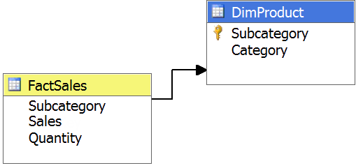
To consider how Analysis Services goes about this, let’s use a very simple cube. In this cube, we are focused on forecasting sales of products. There is one dimension, Product, and it has two attributes, Product Category and Product Subcategory, the latter of which rolls up into the former. In the cube’s one measure group, we have two measures, Sales (Amount) and Quantity, both of which aggregate by simple summation.
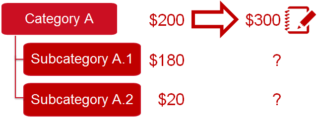
Let’s say that from a previous forecasting exercise, Sales for Subcategory A.1 was expected to be $180 and Subcategory A.2 was expected to be $20 giving us forecasted sales of $200 for Category A.
Two-hundred dollars seems a bit low for Category A so we write a value of $300 to its Sales measure. What should be the new Sales Amount values for subcategories A.1 and A.2?
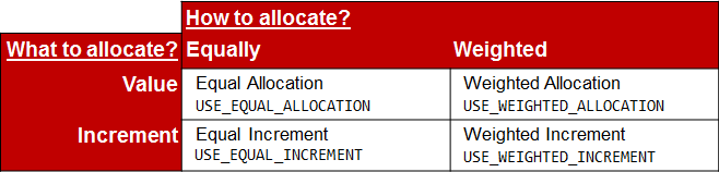
Analysis Services provides you four options for handling this. These options represent the intersection of the answers to two simple questions:
- What would you like to allocate?
- How would you like to allocate it?
The answer to the question of what to allocate is either the value you wrote or the difference between that value the previous value. In our sales forecast example, the value is $300 and the increment – the difference between the new value and the previous value – is $100.
Using either the value or the increment, we now consider how to allocate it. Here we have two options. We can evenly divide the value or increment evenly across the leaf-level members under us – in our case that would be subcategories A.1 and A.2. Or, we can employ a weighting expression to determine which proportion of the value or increment is applied to each leaf member. (This is referred to as weighted allocation.)
NOTE I’m saying “leaf-level member” as I think it’s the easiest for most folks to digest but in reality Analysis Services is considering the leaf-level tuples that aggregate to the tuple to which we are writing. For the very, very simple cube we are using, the two phrases are highly interchangeable. For more complex cubes, understanding the difference in these concepts might be helpful. But then again, that’s probably more technical than most folks need.
The weighting expression is certainly the more complex of these two options but it gives you far more control over the allocation process. The expression is an MDX expression that is evaluated for each leaf-level member. Typically, the weighting expression is calculated as a ratio between 0 and 1 and the sum of all of its evaluations across the leaf-level entries sums to 1. However, neither of these constraints is enforced. This gives you maximum flexibility but also means you need to carefully consider (and validate) your weighting expressions.
The default weighting expression (when weighted allocation is employed but no expression is provided) performs a proportional allocation based on the leaf-level member’s contribution to the original value that is now being overwritten. In our sales example, a proportional allocation would assign 0.90 as the weighting value to Subcategory A.1 as that subcategory’s value of $180 represents 90% of Category A’s value of $200. Similarly, Subcategory A.2 would be assigned a weighting value of 0.10. An equivalent weighting expression would look something like this:
([Measures].[Sales], [Product].[Product Subcategory].CurrentMember) /
([Measures].[Sales], [Product].[Product Category].CurrentMember)
NOTE There are so many ways you can write this expression, and I have purposefully added otherwise unnecessary elements in order to give is a bit more clarity. (If you are new to MDX, clarity is relative, eh?)
Getting back to the questions of what to allocate and how to allocate it, you can now see how we arrive at Analysis Service’s four options for handling allocation. The keyword controlling the allocation behavior is presented in the chart below. This keyword is tacked onto the end of the UPDATE CUBE statement (followed by the weighting expression if one of the weighted options is employed and other than a proportional allocation is desired). If no keyword is provided and allocation must be performed, Analysis Services uses the USE_EQUAL_ALLOCATION option which allocates the value equally amongst the leaves.
To ensure these four options are crystal clear, let’s return one last time to the sales forecast example. We had an original value of $200 for the Category A sales which was the sum of $180 for Subcategory A.1 and $20 for Subcategory A.2. We then updated the sales for Category A from $200 to $300. That gives us a new value of $300 and an increment of $100.
If we perform an even allocation of the value (USE_EQUAL_ALLOCATION), Subcategory A.1 becomes $150 ($300/2 leaves) and Subcategory A.2 becomes $150 ($300/2 leaves). If we perform an even allocation of the increment (USE_EQUAL_INCREMENT), Subcategory A.1 becomes $230 ($180 + $100/2 leaves) and Subcategory A.2 becomes $70 ($20 + $100/2 leaves).
If we perform a weighted allocation of the value (USE_WEIGHTED_ALLOCATION) and use the default weighting expression, Subcategory A.1 becomes $270 ($300 * $180/$200) and Subcategory A.2 becomes $30 ($300 * $20/$200). If we perform a weighted allocation of the increment (USE_WEIGHTED_INCREMENT) and again use the default weighting expression, Subcategory A.1 becomes $270 ($180 + $100 * $180/$200) and Subcategory A.2 becomes $30 ($20 + $100 * $20/$200).
NOTE When the default weighting expression is used, the resulting values are the same even though they are derived using differing logic.
Before leaving the topic of allocations, there are three final items I need to briefly address. First, allocation always occurs at the leaf-level and is aggregated back up. As a result, there can be an accumulation of rounding errors which cause you to get back a value slightly different from the one you wrote. If this is a problem, consider writing to the leaf-levels yourself where you can have explicit control of your values.
Second, some older documentation on allocation in Analysis Services highlights a NO_ALLOCATION option. I’m not sure the story behind it but please be aware there is no such supported option. Some folks say it is accepted in older versions but doesn’t do what’s expected and others say it causes an error to be returned. Either way, don’t use this.
Finally, the Update Isolation Level connection string parameter can be used to improve Analysis Service’s performance during allocation. That said, don’t use it unless you really need it and only use it if you fully understand its impact. I might write a longer entry on this parameter in the future, but for now here’s the short version: setting this parameter to 1 tells Analysis Services that there is no overlap between the cells impacted by allocation in a single UPDATE CUBE statement. This allows Analysis Services to skip some steps it might otherwise perform (which boosts performance). But these steps are also used to ensure you get the right values back from the cube so again don’t use this unless you really need it and you fully understand it.
NOTE There really is a fourth thing I need to address, and that’s around a special leaf-level member in a parent-child hierarchy and how it is handled during allocation. But that’s a topic for another entry.