Measuring Model Goodness - Part 1
Author: Dr. Ajay Thampi, Lead Data Scientist
Data and AI are transforming businesses worldwide from finance, manufacturing and retail to healthcare, telecommunications and education. At the core of this transformation is the ability to convert raw data into information and useful, actionable insights. This is where data science and machine learning come in.
Building a good and reliable machine learning system requires us to be methodical by:
- understanding the business needs
- acquiring and processing the relevant data
- accurately formulating the problem
- building the model using the right machine learning algorithm
- evaluating the model, and
- validating the performance in the real world before finally deploying it
This entire process has been documented as the Team Data Science Process (TDSP) at Microsoft, captured in the figure below.

This post, as part of a two-part series, is focused on measuring model goodness, specifically looking at quantifying business value and converting typical machine learning performance metrics (like precision, recall, RMSE, etc.) to business metrics. This is typically how models are validated and accepted in the real world. The relevant stages of the process are highlighted in red in the figure above. Measuring model goodness also involves comparing the model performance to reasonable baselines, which will also be covered in this post. To illustrate all of this, two broad classes of machine learning problems will be looked at:
- Classification: Covered in Part 1
- Regression: To be covered in Part 2
Classification
Classification is the process of predicting qualitative or categorical responses [source]. It is a supervised machine learning technique that classifies a new observation to a set of discrete categories. This is done based on training data that contains observations whose categories are known. Classification problems can be binary in which there are two target categories or multi-class in which there are more than two mutually exclusive target categories.
In this post, I will look at the binary classification problem taking breast cancer detection as a concrete example. I will be using the open breast cancer Wisconsin dataset for model building and evaluation. The techniques discussed below can easily be extended to other binary and multi-class classification problems. All the source code used to build and evaluate the models can be found on Github here.
Let’s first understand the business context and the data. Breast cancer is the most common cancer in women and is the main cause of death from cancer among women [source]. Early detection of the cancer type — whether it is benign or malignant — can help save lives by picking the appropriate treatment strategy. In this dataset, there are 569 cases in total out of which 357 are benign (62.6%) and 212 are malignant (37.4%). There are 30 features in total, computed from a digitised image of a biopsy of a breast mass. These features describe the characteristics of the nuclei like radius, texture, perimeter, smoothness, etc. The detection of the type of cancer is currently being done by a radiologist which is time consuming and the business need is to speed up the diagnosis process so that the appropriate treatment can be started early. Before diving too deep into the modelling stage, we need to understand the value/cost of making the right/wrong prediction. This information can be represented using a value-cost matrix as shown below:

The rows in the matrix represent the actual class and the columns represent the predicted class. The first row/column represents in the negative class (benign in this case) and the second row/column represents the positive class (malignant in this case). Here's what each of the elements in the matrix represents:
- Row 0, Column 0: Value of predicting the negative class correctly
- Row 0, Column 1: Cost of predicting the positive class wrongly
- Row 1, Column 0: Cost of predicting the negative class wrongly
- Row 1, Column 1: Value of predicting the positive class correctly
For breast cancer detection, we can define the value-cost matrix as follows:
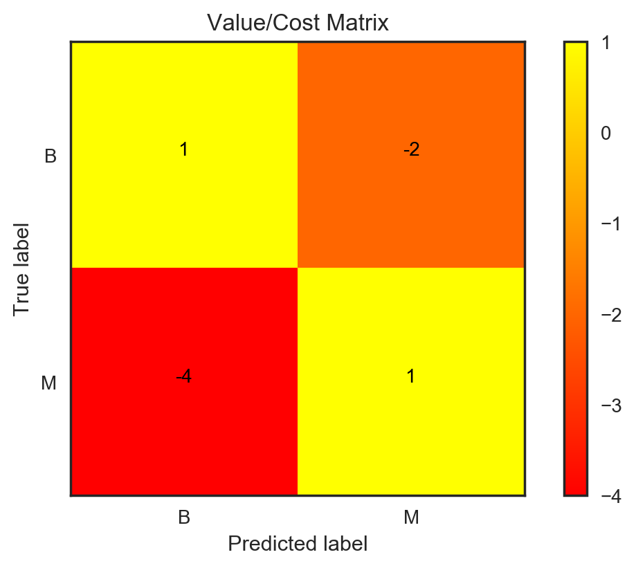
- Detecting benign and malignant cases correctly are given equal and positive value. Although the malignant type is the worse situation to be in for the patient, the goal is to diagnose early, start treatment and cure both types of cancer. So, from a treatment perspective, detecting both cases accurately have equal value.
- The cost of flagging a malignant case as benign (false negative) is much worse than flagging a benign case as malignant (false positive). Therefore, the false negative is given a cost of -4 and the false positive is given a cost of -2.
Another business need is to automate as much of the process as possible. One way of doing this is to use the machine learning model as a filter, to automate the detection of simpler benign cases and only flag the possible malignant cases for the radiologist to review. This is shown in the diagram below. We can quantify this business need by looking at the % of cases to review manually (denoted as x in the figure). Ideally, we want to automate everything without requiring the human in the loop. This means that the model should have 100% accuracy and x should be equal to the actual proportion of positive classes.

After the business needs are properly quantified, the next step is to define reasonable baselines to compare our models to.
- Baseline 1: Random classifier that decides randomly if the cancer type is benign / malignant
- Baseline 2: Majority-class classifier that picks the majority class all the time. In this case, the majority class is benign. This strategy would make much more sense if the classes were heavily imbalanced.
We could add a third baseline which is the performance of the radiologist or any other model that the business has currently deployed. In this example though, this information is not known and so this baseline is dropped.
Now comes the fun part of building the model. I will gloss over a lot of the detail here, as an entire post may be necessary to go through the exploratory analysis, modelling techniques and best practices. I used a pipeline consisting of a feature scaler, PCA for feature reduction and finally a random forest (RF) classifier. 5-fold cross validation and grid search were done to determine the optimum hyperparameters. The entire source code can be found here.
Once the models are trained, the next step is to evaluate them. There are various performance metrics that can be used but, in this post, I will go over the following 6 metrics as they can very easily be explained, visualised and translated into business metrics
- True Positives (TP) / True Positive Rate (TPR) : Number of correct positive predictions / Probability of predicting positive given that the actual class is positive
- False Negatives (FN) / False Negative Rate (FNR) : Number of wrong negative predictions / Probability of predicting negative given that the actual class is positive
- True Negatives (TN) / True Negative Rate (TNR) : Number of correct negative predictions / Probability of predicting negative given that the actual class is negative
- False Positives (FP) / False Positive Rate (FPR) : Number of wrong positive predictions / Probability of predicting positive given that the actual class is negative
- Precision (P) : Proportion of predicted positives that are correct
- Recall (R) : Proportion of actual positives captured
All these metrics are inter-related. The first four can be easily visualised using a ROC curve and a confusion matrix. The last two can be visualised using a precision-recall (PR) curve. Let's first visualise the performance of the model and the baselines using the ROC and PR curves.
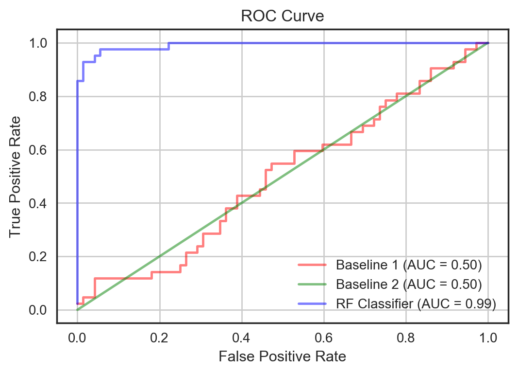
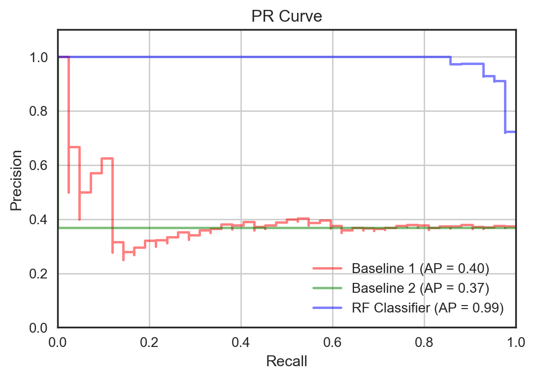
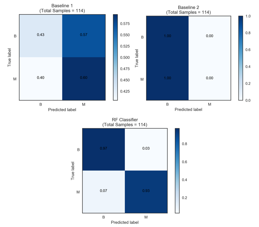
Both plots show the performance of the models using various thresholds to determine the positive and negative classes. As can be seen, the RF classifier outperforms the baselines in every respect. Once the appropriate threshold is picked, we can plot the normalised confusion matrices as shown below. These matrices show the conditional probabilities of predicted values given the actual value. We can see that the baselines do quite poorly especially in predicting the positive class — the false negative rates are quite high. The RF classifier, on the other hand, seem to get much more of the positive and negative class predictions right achieving a TPR of 93% and TNR of 97%.
Now that we’ve established that the new RF model outperforms the baselines, we still need to make sure that it meets our business objectives. i.e. high positive business value and fewer cases to review manually. We therefore need to translate the above performance metrics into the following:
- Total expected value/cost of the model
- % of cases that need to be reviewed manually
The first business metric can be computed by taking the dot product of the flattened confusion matrix (normalised by the total number of samples, S) with the flattened value-cost matrix. This is shown below.
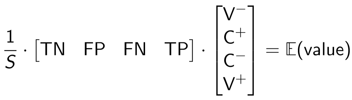
Note that S is a scalar equal to TN + FP + FN + TP. The expected value is essentially the weighted average of the values/costs, where the weights are the probabilities of each of the four outcomes [source].
The second business metric can be computed using precision and recall as follows.

The positive class rate is known from the data used to evaluate the model, i.e. the test set. Based on the business needs, we then need to decide how much of those positive classes we must accurately determine, i.e. the recall. If we want to detect all the positive cases, the target recall should be 100%. We can then find the corresponding precision (and threshold) from the PR curve. For the ideal model with 100% precision and recall, the proportion of positive cases to review would be equal to the actual positive class rate. This means we could, in theory, achieve 100% automation without a human in the loop.
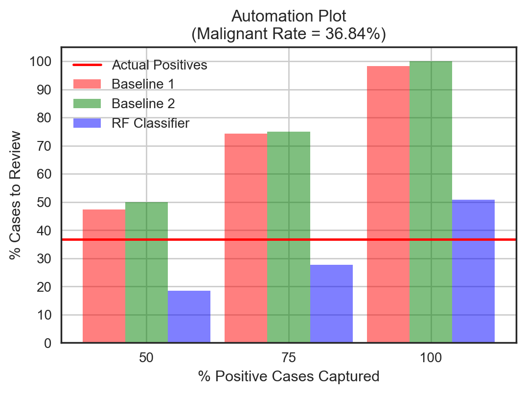
The following two plots show the final evaluation of the model goodness in terms of the two key business metrics.
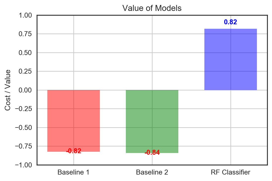
Observations:
- Both baseline models have quite large costs because of the high false negatives. The random forest classifier has a good positive value by getting a lot of the positive and negative cases right.
- For the case of breast cancer detection, we want to capture all the positive/malignant cases, i.e. 100% recall. Looking at 50% or 75% recall does not make sense in this example because of the high cost of not treating the malignant cases. For other binary classification problems like fraud detection for instance, a lesser recall may be acceptable so long as the model can flag the high cost-saving fraudulent cases. Regardless, we can see that the RF classifier outperforms the baselines on the automation front as well. To capture 100% of the malignant cases, the radiologist would only need to review about 50% of all cases, i.e. 13% additional false positives, whereas he/she would have to review almost all the cases using the baseline models.
In conclusion, the first part of this series has looked at measuring model goodness through the lens of the business, specifically looking at classification-type problems. For further details on this subject, the books below are great references. In the second and final part of this series, I will cover regression which requires looking at slightly different metrics.
Further Reading
- Elements of Statistical Learning, by Trevor Hastie, Robert Tibshirani, Jerome Friedman
- Data Science for Business, by Foster Provost and Tom Fawcett
- Hands-On Machine Learning with Scikit-Learn and Tensorflow, by Aurélien Géron