Analysing data in SQL Server 16, combining R and SQL

Article
08/01/2016

By Michele Usuelli, Data Scientist Consultant

Overview

R is the most popular programming language for statistics and machine learning, and SQL is the lingua franca for the data manipulation. Dealing with an advanced analytics scenario, we need to pre-process the data and to build machine learning models. A good solution consists in using each tool for the purpose it's designed for: the standard data preparation using a tool supporting SQL, the custom data preparation and the machine learning models using R.

SQL Server 2016 has the option to include an extension: Microsoft R Services. It's based on MRS (Microsoft R Server), a tool designed by Revolution Analytics to scale R across large data volumes. In SQL Server 2016, R Services provides a direct interface between MRS and the SQL databases. In this way, it's possible to analyse the SQL tables and to create new tables using the MRS tools. In addition, the R package RODBC allows to run SQL queries from R.

This article shows a simple example integrating R and SQL. To follow all the steps, some prior knowledge about the basic R functions is required.

Setting-up the environment

In this article, we are using a SQL Server 2016 VM. To set-up the environment, the steps are

Log-in to Azure and set-up a SQL Server machine with R Services. To install R Services, refer to this: https://msdn.microsoft.com/en-us/library/mt696069.aspx
Connect to SQL Server: from the Windows task bar, open SQL Server Management Studio and connect to it using your credentials.
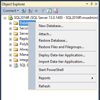
Create a new database: right-click on Databases and choose New Database… .
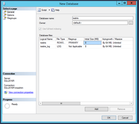
Give a name to the new database, e.g. iristest. Then, click on Add and OK.
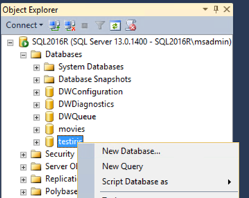
Open the query editor: right-click on the new database and choose New Query.
Define the credentials to authenticate to the database: in the editor, paste and run the following query. You should replace the parameter testiris with the name of your database, and username and password with new credentials to access this database.

USE [testiris]
GO
CREATE LOGIN [username] WITH PASSWORD='password', CHECK_EXPIRATION=OFF,
CHECK_POLICY=OFF;
CREATE
USER [username] FOR LOGIN [username] WITH DEFAULT_SCHEMA=[db_datareader]
ALTER
ROLE [db_datareader] ADD
MEMBER [username]
ALTER
ROLE [db_ddladmin] ADD
MEMBER [username]

Build a new RStudio or Visual Studio project and create a new R script. See https://www.rstudio.com/products/RStudio/
Define a list with the parameters to connect to the database. They should be the same as in the previous SQL query.

sql_par <-
list(

Driver =
"SQL Server",

Server =
".",

Database =
"testiris",

Uid =
"username",

Pwd =
"password"
)

Starting from the list of parameters, define a connection string for the SQL database. For this purpose, you can use the function paste.

sql_connect <-
paste(names(sql_par), unlist(sql_par),

sep =
"=", collapse =
";")

Define a MRS data source object containing the information to access the iristest database. The inputs are the table name, e.g. iris, and the connection string.

table_iris <- "iris"
sql_iris <-
RxSqlServerData(connectionString = sql_connect,

table = table_iris)

Import the data into a SQL table. For this purpose, we can use rxDataStep. Its inputs are the local dataframe iris, the data source object sql_iris, and overwrite = TRUE, specifying that we are overwriting the table if existing already. To avoid issues in the SQL queries, we also re-name the columns of iris, replacing the . with an *_*.

names(iris) <-
gsub("[.]", "_", names(iris))
rxDataStep(iris, sql_iris, overwrite =
TRUE)

## Rows Read: 150, Total Rows Processed: 150, Total Chunk Time: Less than .001 seconds

Install and load the package RODBC and initialise it using the connection string. We define the object channel containing the information to access the database.

library(RODBC)
channel <-
RODBC::odbcDriverConnect(sql_connect)

Exploring the data

To explore the data, we can either use MRS or SQL. In MRS, there is the option to quickly access the metadata using rxGetVarInfo.

rxGetVarInfo(sql_iris)

## Var 1: Sepal_Length, Type: numeric, Low/High: (4.3000, 7.9000)
## Var 2: Sepal_Width, Type: numeric, Low/High: (2.0000, 4.4000)
## Var 3: Petal_Length, Type: numeric, Low/High: (1.0000, 6.9000)
## Var 4: Petal_Width, Type: numeric, Low/High: (0.1000, 2.5000)
## Var 5: Species
## 3 factor levels: setosa versicolor virginica

The output contains the name and type of each field. Also, it's possible to compute a quick summary of the table using rxSummary. The inputs are

Formula: what variables we want to summarise, using the formula syntax. For more info about the formula, have a look at the related material typing ?formula into the R console. To include all the variables, we can use . .
Data: the data source object, containing the information to access the data.

summary_iris <-
rxSummary(~ ., sql_iris)

## Rows Read: 150, Total Rows Processed: 150, Total Chunk Time: Less than .001 seconds
## Computation time: 0.005 seconds.

summary_iris$sDataFrame

## Name Mean StdDev Min Max ValidObs MissingObs
## 1 Sepal_Length 5.843333 0.8280661 4.3 7.9 150 0
## 2 Sepal_Width 3.057333 0.4358663 2.0 4.4 150 0
## 3 Petal_Length 3.758000 1.7652982 1.0 6.9 150 0
## 4 Petal_Width 1.199333 0.7622377 0.1 2.5 150 0
## 5 Species NA NA NA NA 150 0

This summary contains some basic statistics like the mean and the standard deviation.

Using RODBC, we can run any SQL query. The inputs are the connection object channel, defined previously, and the query string. Let's see a simple example.

RODBC::sqlQuery(channel, "select count(*) from iris")

As expected, the output is the number of records.

R contains good string manipulation tools that allow us to build complex queries and to write extensions. To show the approach, we perform a simple group by operation. The steps are

Define the skeleton of the query, leaving the column names as %s parameters
Define the parameters
Define the query inclusive of its parameters using sprintf
Run the query

The R code is

query_sql <- "select %s, avg(%s) as avg_sl from iris group by %s"
col_group <- "Species"
col_value <- "Sepal_Length"
query_count <-
sprintf(query_sql, col_group, col_value, col_group)
df_avg_value <-
RODBC::sqlQuery(channel, query_count)
df_avg_value

##
## Attaching package: 'dplyr'

## The following objects are masked from 'package:stats':
##
## filter, lag

## The following objects are masked from 'package:base':
##
## intersect, setdiff, setequal, union

## Species avg_sl
## 1 setosa 5.006
## 2 versicolor 5.936
## 3 virginica 6.588

Using a similar approach, we can define more complex queries. Also, if we need to run similar queries many times, it's possible to build R functions that build the query depending on some given parameters.

Processing the data

To process the data, it's possible to use both MRS and SQL. With MRS, we can process the data using the function rxDataStep. This function allows to build custom data processing operations. A simple example consists in defining a new column Sepal.Size with simple maths operations. The steps are

Define a new SQL data source object
Define the SQL table using RxSqlServerData. Its arguments are the input and output data object, and overwrite = TRUE, similarly to before. In addition, we define the new column using the transforms input.
Have a look at the new table using rxGetVarInfo

This is the code:

table_iris_2 <- "iris2"
sql_iris_2 <-
RxSqlServerData(connectionString = sql_connect,

table = table_iris_2)
rxDataStep(inData = sql_iris,

outFile = sql_iris_2,

transforms =
list(Sepal.Size = Sepal.Length *
Sepal.Width),

overwrite =
TRUE)
rxGetVarInfo(sql_iris_2)

## Rows Read: 150, Total Rows Processed: 150, Total Chunk Time: Less than .001 seconds

As expected, we have a new column: Sepal_Size.

Using the same approach, it's possible to build complex custom operations, making use of the open-source R functions.

Using RODBC, it's possible to run an SQL query defining a new table. For instance, we can join two tables. Using an approach similar to the previous SQL query, we build the related string and execute it using RODBC.

table_avg_value <- "avg_value"
sql_avg_value <-
RxSqlServerData(connectionString = sql_connect,

table = table_avg_value)

rxDataStep(df_avg_value, sql_avg_value, overwrite =
TRUE)
query_join <- "select Sepal_Length, Species from iris
left join avg_value
on iris.Species = avg_value.Species"
df_join <-
RODBC::sqlQuery(channel, query_join)
df_join <-
df_join[, c("Sepal_Length", "Species", "avg_sl")]
head(df_join)

## Joining by: "Species"

## Sepal_Length Species avg_sl
## 1 5.1 setosa 5.006
## 2 4.9 setosa 5.006
## 3 4.7 setosa 5.006
## 4 4.6 setosa 5.006
## 5 5.0 setosa 5.006
## 6 5.4 setosa 5.006

After having processed the data, it's possible to build machine learning models starting from the SQL tables. In this way, we don't need to pull the data in-memory and we can deal with a large data volume. For instance, to build a linear regression, we can use rxLinMod. Similarly to rxSummary, the arguments are formula, defining the variables to include, and data, defining the data source. After having built the model, we can explore is using summary, similarly to open-source R.

model_lm <-
rxLinMod(formula = Petal_Length ~
Sepal_Length +
Petal_Width,

data = sql_iris)

## Rows Read: 150, Total Rows Processed: 150, Total Chunk Time: Less than .001 seconds
## Computation time: 0.000 seconds.

summary(model_lm)

## Call:
## rxLinMod(formula = Petal_Length ~ Sepal_Length + Petal_Width,
## data = sql_iris)
##
## Linear Regression Results for: Petal_Length ~ Sepal_Length +
## Petal_Width
## Data: sql_iris (RxXdfData Data Source)
## File name: iris.xdf
## Dependent variable(s): Petal_Length
## Total independent variables: 3
## Number of valid observations: 150
## Number of missing observations: 0
##
## Coefficients:
## Estimate Std. Error t value Pr(>|t|)
## (Intercept) -1.50714 0.33696 -4.473 1.54e-05 ***
## Sepal_Length 0.54226 0.06934 7.820 9.41e-13 ***
## Petal_Width 1.74810 0.07533 23.205 2.22e-16 ***
## ---
## Signif. codes: 0 '***' 0.001 '**' 0.01 '*' 0.05 '.' 0.1 ' ' 1
##
## Residual standard error: 0.4032 on 147 degrees of freedom
## Multiple R-squared: 0.9485
## Adjusted R-squared: 0.9478
## F-statistic: 1354 on 2 and 147 DF, p-value: < 2.2e-16
## Condition number: 9.9855

The output is the same as using open-source R function lm. The difference is that we can apply this function on a large table without needing to pull it in-memory.

Conclusions

SQL and MRS are designed for different purposes. Having them into the same environment, it's possible to use each of them in the most proper context: SQL to prepare the data, MRS to build advanced machine learning models. Also, the string manipulation tools provided by R allow to build SQL queries, making it possible to write code extensions. Another option is to include R code within the SQL queries although we haven't dealt with that in this article.