Why Pay for Sorting if You Don’t Need it? (3 of 3)

By Chen Fu, Tanj Bennett, Ashwini Khade

In our previous posts, we discussed the high cost of data sorting. Here we introduce Venger Index, an alternative option when you need memory efficiency but not data sorting.

1. Venger Index – Balancing Cost and Performance

Hash tables do not require data sorting, and are widely used in memory based data tables. Its use in disk or flash based data stores, however, are limited due to high memory cost. A hash table requires all keys to be in memory. When the key occupies a significant portion of the key-value pair, this cost becomes prohibitive. For instance, in a web document data store, when the URLs are used as keys, the key size can be more than one hundred bytes.

Our goal is to build an index that is at least as memory efficient as the LSM tree. We achieved the goal by modifying the hash table with the following key ideas:

1. Key Hashing. We use md5 to hash original keys to 128 bit integers, same size with GUID. The number of unique keys are so large that the chance of collision can be ignored. We can also extend the key size from 128b to 192b or 256b, without affecting memory cost or performance of the index.
2. Key Folding: In the index, we don't store the full 128b key, but a hashed partial key of 27 bit. This is cheating. We will explain later about how we get away with it, and why 27.
3. Hash Block Spilling. To further save memory, we spill most of the hash entries from memory to the SSD, and only load them to memory when needed. Unlike memory, the main media is not suited for accessing of small items such as one hash entry. Thus we group hash entries into Hash Blocks.

Key folding and hash block spilling will cause performance degradation comparing with standard hash table. Next we explain the structure of the index in detail, and show how we effectively reduce memory usage while keep performance degradation in check.

1.1 Index Architecture

Venger index is designed for a partitioned data store, assuming each machine has 50 to several hundred partitions. Each partition has an instance of the index and a data file. Each record in the data files has a header containing the 128b full key and size of the record. The index maps a record's key to its location in the data file. Each hash entry takes the form <partial_key, size, address>. In our first implementation, the size of this entry is 8 bytes, with 27-bit partial key, 3-bit size and 34-bit address.

The size field is a logarithmic scale representation of sizes from 2k to 128k. For larger records, we treat the sizes as 128k. Using log scale size means that when we read a record, we have to load more data in memory than necessary, causing read amplification, but no larger than 2. For records that are bigger than 128k, we read in 128k first, then consult the size field in the data header to determine how much we missed, and use a second read operation to bring it in. Since it is unlikely the SSD can read the whole 128k in one read operation, we are not increasing read amplification here.

34-bit address can be used to address a data file up to 16GB. If we force all record sizes to align to 64-bit boundary, 34-bit can address 16G number of 64-bit numbers, that's 128GB. With 300 partitions, for example, we can manage up to 38TB of data on a single machine.

We group a fixed number of hash entries into a Hash Block. Each hash block is guarded by one bloom filter and one Shadow Key Block. Currently we fit 512 entries into a hash block that is 4KB in size. One hash block with its corresponding bloom block and shadow key block, is called a Hash Page.

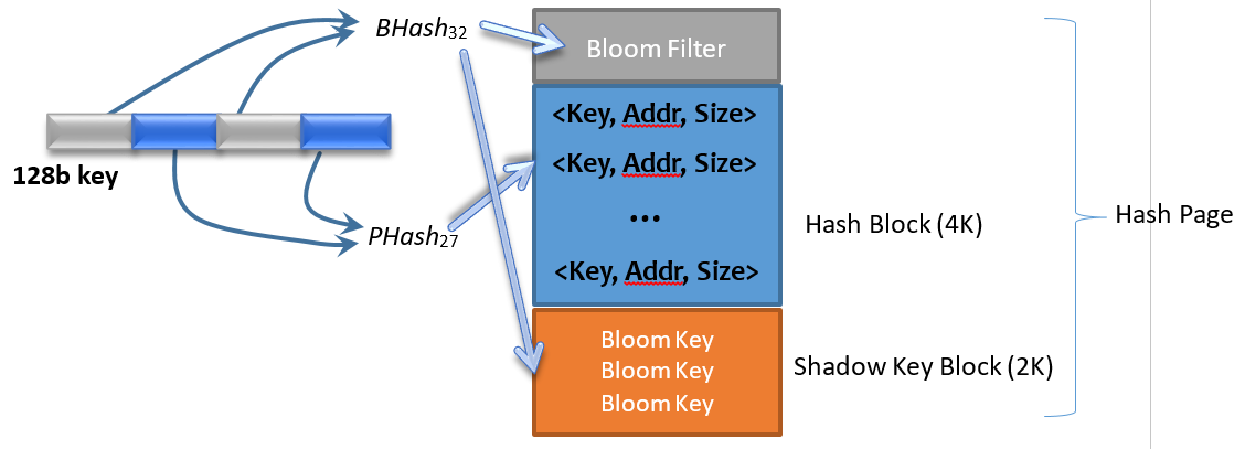
Figure 3 Hash Page Structure

Figure 3 Illustrates how to insert a new 128b full key to a hash page. Two segments of the full key are passed into two hash functions, BHash₃₂ and PHash₂₇, respectively. The first result BHash₃₂(128b_key) is a 32-bit number used as the bloom key, and the second result PHash₂₇(128b_key)  is a 27-bit number used as the partial key. The bloom key is used to populate the bloom filter, and also saved in the Shadow Key Block. The partial key is inserted into the hash block. Here we try to keep the bloom key and the partial key independent from each other, so as to reduce the chance of partial key collision, which will be explained later in Section 1.5. Shadow key blocks are only used during index compaction, explained in Section 1.4.

As shown in Figure 4, each index instance consists of a number of hash buckets (e.g. 1024 for 10M keys). Each bucket is a linked list of hash pages. When 10M keys are divided into 1k buckets, each bucket has 10k keys, that is 20 hash pages since each page has 512 entries.

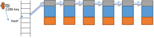
Figure 4 In Memory Index

This configuration still uses too much memory comparing with LSM trees. To further save memory, we spill most of the hash pages to SSD, only keep the head page in memory, as shown in Figure 5.

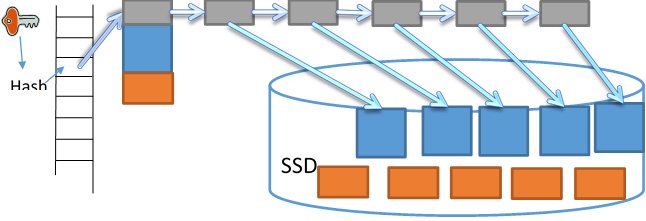
Figure 5 Spilling to SSD

1.2 Adding a new entry:

When a new Key-value pair enters the system, we need to create a new hash entry and insert it into our index. Overwriting of an existing key-value pair is achieved by simply adding a new version. Deleting is also achieved by writing a tombstone entry with the key and empty value. It will become clear after section 1.3, that our index support versioning naturally.

Steps:

1. Write the new key-value pair into the data file
2. Locate the correct bucket by hashing the full 128b key.
3. If the first hash block of the bucket is full,
   1. create a new hash page, insert it into the head of the linked list.
   2. Kick off asynchronous spilling of the second page in the list.
4. Generate keys and populate the keys in the first hash block, according to Figure 3

As we always insert the new entry in to the head page of the linked list, all the entries in a bucket is sorted chronically, with youngest entries near the head of the list. This makes query of the young records faster. Based on our observation, younger records tend to be queried more often than older ones.

1.3 Querying a Key

In this operation, the input is a key, and we need to return the location of the record that matches the key, or "not found" if there is no such key in the index.

First we locate the right bucket by computing the hash of the full 128b key. Next we compute the partial key and the bloom key the same way we do in Figure 3.

Then we traverse the list of hash pages trying to locate the right hash entry. For each hash page on the linked list, we first test the bloom key against the bloom block. If the bloom test is successful, we load the hash block to memory, and then search the block for an entry that matches the partial key, and return the location if found. "Not found" is returned if we reach the end of the linked list without finding a match.

Note that since the partial key produced by PHash₂₇(128b_key)  has only 27 bits, there are cases where multiple full keys are hashed into the same partial key. As a result, there are false matches, when the index returns a result based on partial key match, but the address does not point to the key asked by the client. The caller of this operation must verify the match by reading the full key from the SSD, and ask the index to retry in the case of a false match.

When the caller discovers a false match, it calls the index query API again with the fully key and a "previous address". The index would scan the list of pages again as described above, but this time go pass the entry with the "previous address", and then return the next match.

As shown in Section 1.2, hash entries are ordered chronically in the index. When there are multiple versions of the same key in the index, based on our query algorithm, younger entries are always returned first. However, the client has the option to search for older versions by using the retry mechanism.

There are two things that incur read amplification and hurt performance here. They are, 1) bloom filter false positive induced unnecessary hash block scan, and 2) hash collisions from PHash₂₇(128b_key) , which require us to consult the data file repeatedly. Probability of these two can be reduced by increasing memory usage in the index. We will discuss in Section 1.5 how we precisely tradeoff between performance vs memory usage.

1.4 Relocation and Eviction

Garbage collection is necessary for all key-value store to rid the system of deleted or overwritten records. During garbage collection, the data file needs to rearrange records to allocate space for new coming records. Thus our index must support moving a record from one location to another (relocation), or removing a record (eviction).

For relocation, the caller needs to provide a key, its old location and new location. For eviction, the caller needs to provide a key and its old location. It is simpler to combine these two operations as one, with the latter providing an invalid new location.

Implementation is straight forward, with the full key, we can search the index the same way we described above. However, we won't have false match, as we match not only the partial key, but also the old location. The match is unique since the location is unique.

Once we load the hash block to memory, and located the hash entry with the matching partial key and the old location, we simply update that hash entry in place. And if the new location is invalid, we set the partial key to the invalid value too. This way we get rid of the key from the index. The block needs to be flush to SSD on a later time.

Whenever a hash entry is removed from the index, it leaves an invalid entry in the index, which takes up spaces. Periodical compaction is needed to get rid of invalid entries in the index itself. One way to do this is to create a new linked list of hash pages, copy all the valid entries over, and switch the head pointer of the bucket to point to the new list. When we compacting hash pages, we need to regenerate new bloom filters, using the bloom key saved in the Shadow Key Block (Figure 3). The is the only time when the shadow key blocks are needed in memory.

Note that a relocation operation needs to bring a hash block to memory for updating. And index compaction needs all the hash blocks and shadow key blocks of a bucket in memory. It would be more efficient if these two can be coordinated. When a data file garbage collection starts, it would call relocation multiple times, loading many hash blocks in memory. The index can just keep these blocks in memory until garbage collection finishes, then start index compaction right way. As soon as one bucket is compacted, most hash blocks and shadow key blocks in that bucket can be spilled to SSD.

It seems that we need to load all the hash blocks in memory during garbage collection, defeating all our memory saving efforts. However, since we are in a partitioned data store with more than 50 partitions in a single machine, each partition can take turns performing garbage collection. As long as we keep the number of concurrent garbage collection low, the memory saving is not negated. We will discuss our memory cost in detail next.

We store hash blocks and shadow key blocks on SSD. Index compaction would generate new blocks and makes old ones expire. This causes write amplifications. Suppose we allow 5% of hash entries to be invalid before starting index compaction, and each compaction would rewrite all the blocks on SSD, then the write amplification is 20. On the other hand, since hash entry only accounts for a very small fraction of the data (1% with 1k records, even smaller when records are bigger), damaging effect of the write amplification in the index is very small. We will discuss write amplification of data files later.

1.5 Performance vs. Memory Cost

As described previously, we save memory by sacrificing some performance, e.g. false matching caused by key folding. To ensure a good balance between performance and memory consumption, there are several parameters in the system that can be tuned, including number of buckets, size of the bloom filter and width of the partial key.

Now we use one example setting to illustrate how this is done. Suppose we need to have an index that holds up to 10M keys. We choose the number of buckets to be 1024, thus 10K keys per bucket. 512 hash entries per hash page, so about 20 hash pages per bucket.

As seen from section 1.3, we guard the loading and searching of hash blocks with bloom filters. When searching for a key, we could test 20 bloom filters, each with a false positive rate p. Suppose one goal is to have less than 1% of the queries to scan a hash block that does not contain the desired key. Then we need p to satisfy

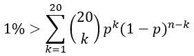And we get p < 0.05% . We can use a 1KB bloom filter (max 512 items) to achieve this. This way, 99% of the read requests can be satisfied by at most two reads to the SSD, one read to load a hash block, a second read to load the requested data record (except records larger than 128k). 99.995% of the read requests can be satisfied by at most 3 reads.

Now consider the probability of a false matching. Assuming we can find a good quality hash function (output follow uniform distribution) to produce the partial keys, then:

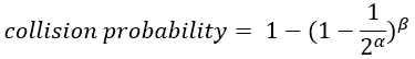
where α is the size of the partial key, and β is the number of hash entries checked in a query. Since hash blocks are guarded by bloom filters, 99.995% of queries only need to query 1 or 2 hash blocks. It is safe to assume that in vast majority of the cases, β to be smaller than 1024 (two hash blocks), in which case an α of 27 leads to a false match probability less than 0.01%.

Based on this example, in an index with 10M hash entries, we have 20k hash pages. We need 20k bloom filters in memory, occupying 20MB. Accounting for all the head pages of the buckets, we have 1K hash blocks and shadow key blocks in memory, occupying 6MB. That's 2.6 byte per key memory cost.

During garbage collection, the rest of the hash blocks are brought in memory, which is 76MB. For shadow key blocks used during index compaction, we only need one bucket at a time, 38KB. If we perform garbage collection on 2% of the data files, average cost is 1.5MB. Overall, Venger Index has a memory cost of 2.8 byte per key.

Note that most of the memory cost comes from the bloom filters, which we use just the standard implementation. Replacing it with more advanced implementations such as perfect hashing would lead to even more memory saving without sacrificing performance.

2. Data Files

Based on the description above, the Venger Index only requires two things from the data file, 1) 34b addressable, and 2) to be notified of garbage collection start and end. It does not need to know how data are organized inside a data file, leaving a lot of room to improve write amplification. Below are two example implementations of data files.

2.1 Circular Data File

A simple layout is a logical circle. A continuous portion of the circle contains the data, as shown in Figure 6. New records are always appended at the tail end. A garbage collector reads from head of the data, discarding expired or deleted records, and rewrite the alive records at the tail end. As both the new data and the old data are appended at the tail end, the garbage collector slowly mixes new data with old, like kneading a dough. Overtime, different age records are distributed at different places on the circle.

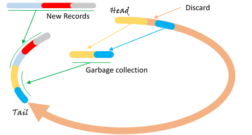
Figure 6 Circular Data File

Write amplification induced by the garbage collector depends on portion of the obsolete data in the data file. If we allow 10% of obsolete data in the store, assuming the data file is 10G, then one scan of the entire file rewrites 9G of the existing data, to make room for 1G of new records, resulting a write amplification of 10. Obviously more extra space would result in lower write amplification.

2.2 Multi-Stream Data File

A problem with the circular file is mixing of records with different time to live (TTL). The garbage collector has to constantly rewrite living records while discarding dead ones. If we know the TTL of each record, then we can group data records together that are likely to die at the same time, thus further reduce write amplification.

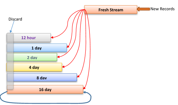
Figure 7 Multi-Stream

We are implementing a new multi-stream data file, illustrated in Figure 7. Here we assume that we know the TTL for each record; delete and overwrite (operations that shorten TTL unexpectedly) are rare, or mostly happen to fresh data.

Here a single data file is split into multiple logic streams. Each stream is a list of physical SSD pages forming a logical belt that can grow and shrink dynamically. The tail page can be in memory to avoid fragmentation. The new records are appended to the tail end of the fresh stream. A garbage collector picks records from the head of the fresh stream, and append them to a stream's tail end based on the record's remaining TTL. It also discards expired records from each streams' head, freeing up spaces. Except for the last stream, where alive records are again appended to the tail.

This way, we use the fresh stream to catch deletions and overwrites to fresh records. And for records that survive fresh stream, and live shorter than two weeks, we have write amplification only 2. A long living record are rewritten once every two weeks. For data sets with no deletion or overwriting (e.g. event logs), we can skip the fresh stream and get rid of write amplification.

3. Conclusion

Here we present Venger Index, an alternative option to LSM tree for a storage system, when memory efficiency is required, but data sorting is not. Removing data sorting leads to reduced I/O cost, and prolonged SSD life. At the same time, hash based index can effetely reduce load unbalancing, a valuable property in large scale distributed storage systems.

Venger Index is implemented as part of Exabyte Store, open sourced Key-Value pair storage engine.