Azure Machine Learning – First Look

Article
10/01/2014

An intriguing new Azure-based service was recently announced that has an opportunity to be a game changer in the business analytics space. This service, known as Azure Machine Learning opens the door to enterprise-strength data science in a managed environment without requiring a PhD. By lowering the bar and democratizing machine learning a new class of business analyst is invited in. Make no mistake however, this doesn’t mean it isn’t an industrial quality machine learning platform.

In this blog, we will take a whirlwind tour of the Azure Machine Learning service, starting first with the creation of a new experiment. From our experiment, we will train a machine learning model and subsequently expose this model by an endpoint to allow for integration into a LOB or other application.

Getting Started

The Azure Machine Learning Services is currently in preview and is available in your Microsoft Azure Portal. Before you can get started with these experiments, you will need to create and configure your workspace. Once your workspace is created, you will have access to ML Studio, which is the tool used for the remainder of this blog. This process is relatively self-explanatory and step-by-step walk-through is beyond the scope of this blog.

A Familiar Example

If you’ve done any amount of business intelligence or analytics work on the Microsoft SQL Server platform, you’ve inevitably seen or played with the Adventure Works SQL Server Analysis Services data mining examples. In this first look, we are going to take that familiar and well-worn example and port it to the new Azure Machine Learning services. To start this example, you will need to create a CSV export of the dbo.vTargetMail view found in the AdventureWorks Data Warehouse sample db. For your convenience I have include the SQL statement, I used for my demo below.

 SELECT
    Gender,YearlyIncome,TotalChildren,NumberChildrenAtHome,
    EnglishEducation,EnglishOccupation,HouseOwnerFlag,
    NumberCarsOwned,CommuteDistance,Region,Age,BikeBuyer
FROM [dbo].[vTargetMail]

Building the Experiment

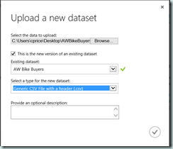
Before starting this new experiment, we must first upload the dataset. After launching ML Studio, click the ‘+ New’ button and then Dataset and finally ‘From Local File’. In the ‘Upload’ dialog, select the CSV file you created on your local file system, specify a name for the data set (AW Bike Buyer) and set the appropriate type. Since our example data is a CSV with a header row, I used the ‘Generic CSV File with a header (*.csv)’ type.

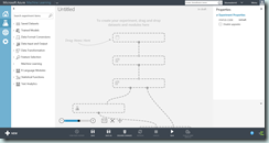
Once the upload is complete, we are ready to get started with our experiment. Again, using the ‘+ New’ button, select Experiment to create a new , empty experiment workspace. Before we build the experiment, let’s familiarize ourselves with the landscape of ML Studio.

ML Studio Overview

Within the context of an experiment, ML Studio consist of four parts:

The experiment items found in the left panel is organized by category and includes a search to easily locate different items.
The properties window found in the right panel allows for configuration of individual experiment items.
The experiment design surface where items are added and wired or orchestrated together. At the bottom of the design surface are controls to zoom, pan and otherwise navigate the experiment.
Finally, at the bottom is the tool bar, where you will save, refresh and run your experiment when ready.

A Simple Experiment

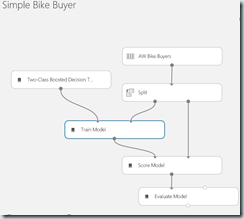
In just 6 steps, we can build a simple straight-forward experiment. Create a new experiment, name it appropriately (Simple Bike Buyer) and then use the following steps:

Add the ‘AW Bike Buyer’ data set from the list of Saved Datasets to the design surface.
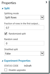
To train and test (or score) or experiment, we will need to split the data set into two parts. Search for and add the Split item (Data Transformation >> Sample and Split) to the experiment then connect the output from the data set to the input of the split. The default for the Split item, is a 50% random split. For this experiment, change the ‘Fraction of rows in first output’ property in the Properties window from 0.5 to 0.7. This will allow us to use 70% of the data for training our model and 30% for testing. Note as you are wiring up your experiment, you get green and red visual indicators which help you know types each input or output expects.
Now we need to initialize a machine learning model. For this experiment we will use the Two-Class Boosted Decision Tree model (Machine Learning >> Initialize Model >> Classification). Find and add this item to the design surface.
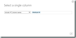
Next we must train our selected model using the Train Model (Machine Learning >> Train) item. After adding the item to the experiment, connect the output from the Two-Class Boosted Decision Tree model to the first input of the Train Model. The first output of the Split (the 70%)created in step 2, is then wired to the second input. Once wired, launch the Column Selector in the properties window. In order to train the model, we need to tell the item which column we would like to predict. Ensure ‘Column Name’ is selected and type ‘BikeBuyer’ as seen in the screen shot below.
After training the model, we need to score it using the Score Model (Machine Learning >> Score) item. Search and add Score Model and then wire the output from the Train Model to the first input and the second output from the Split (the 30%) which has our test cases into the second input.
Finally, we use the Evaluate Model (Machine Learning >> Evaluate) item to visual the results of out experiment. Once added, this item accepts the output from the Score Model into the first input. For now ignore the second input, which we will explore in a future blog post.

When the resulting experiment looks similar to the screenshot above., your are ready to run the experiment. In the toolbar, click the ‘Run’ button. Your experiment will be queue and run within the Azure Machine Learning cloud service. As your experiment progresses you will notice green checkmarks appear on the various items in your experiment. After the experiment is finished running, you can explore the results.

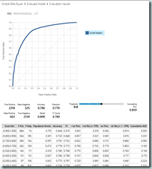
On the Evaluate Model item, right-click the output connector and select the Visualize item from the context menu. The results of your experiment are presented in the form of a ROC curve as well as metrics such as Accuracy, Recall, Precision and F1 score that are used to evaluate the usefulness of the model.

What’s Next

With that you’ve created your first experiment and while you will note that this model didn’t perform particularly well out of the box, we’ve only scratched the surface. In subsequent blog posts we will iteratively refine and expand on this example by evaluating other models and tuning both the data and algorithm to deliver a more useful result. Once we find a suitable model, we will expose it as a web service for consumption.

Till next time!