What’s new for SQL Server 2016 Analysis Services in CTP3.2
What is new in SQL Server Analysis Services 2016 CTP3.2
Just a few weeks after releasing SQL Server Analysis Services 2016 CTP3.1, we are delivering a new update to Analysis Services again. This month’s updates are focused on tabular models at the 1200 compatibility level and include scripting in SSMS, calculated tables, and DirectQuery.
Scripting the new 1200 compatibility level models
With CTP 3.2 you can use scripting for models set to the new 1200 compatibility level in SSMS. Scripts use the JSON-based format already introduced in the BIM file, only now also extended with commands. SSMS generates object definitions in JSON; the Analysis Services engine understands this format natively.
Before we continue, let’s talk a bit about terminology and how JSON fits into the existing architecture. In Analysis Services we have a few concepts that are important to the discussion:
- XMLA: XML for Analysis (XMLA) is a Simple Object Access Protocol (SOAP)-based XML protocol, designed specifically for universal data access to any standard analytical data source residing on the Web.
- ASSL: Applications maintain and administer Analysis Services using the XML-based Analysis Services Scripting Language (ASSL). ASSL extends XMLA to represent the object definition language for multidimensional objects like cube, dimension, and measuregroup to describe parts of a model.
[* Many people will use the term XMLA to include ASSL even though they are technically different.]
Until now ASSL has been used for both multidimensional and tabular databases. With CTP 3.2, we introduce the JSON-based Tabular Model Scripting Language (TMSL).
Functionally, TMSL is equivalent to ASSL and is used for Tabular models at the 1200 compatibility level. Just like ASSL is executed over the XMLA protocol, so is TMSL. This means that the XMLA.Execute method now takes JSON-based scripts (TMSL) in addition to the XML-based scripts (ASSL) as part of the payload.
With our terms defined, let’s take a look at the difference between the script generated for a table with partitions for a ASSL-based 1103 tabular model versus the new TMSL JSON-based 1200 model.
Here is a table with 3 partitions:
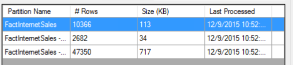
Scripting out a single partition using ASSL gives us 28 lines of script that references objects like MeasureGroups, Cubes, and even ProactiveCaching -- features and concepts foreign to the Tabular model.
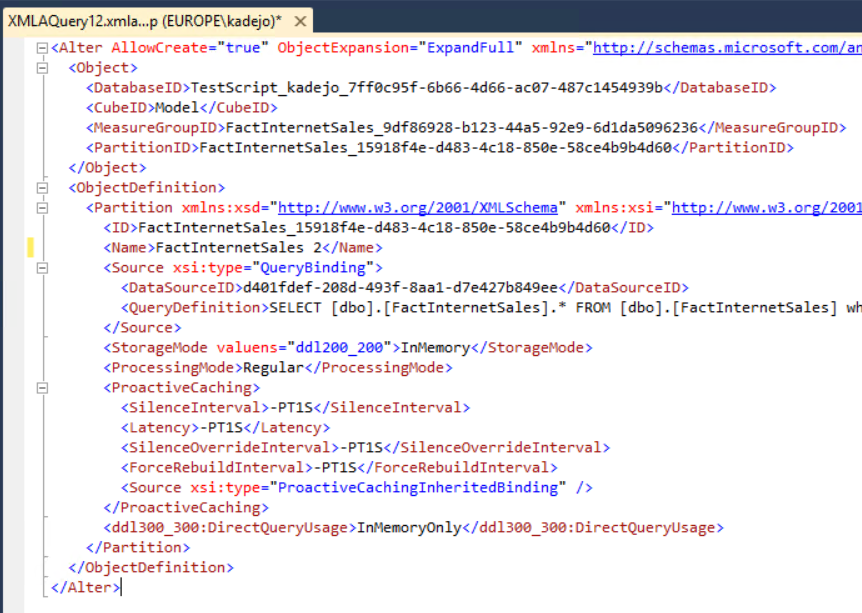
As you can see, this script doesn’t really reflect the natural representation of the tabular model.
After upgrading the model to the new 1200 compatibility level and scripting it again, we see the new TMSL script:
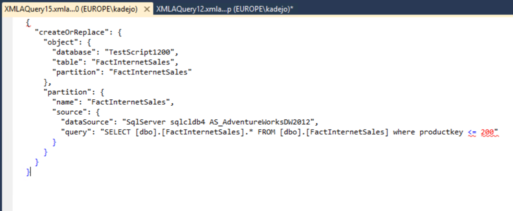
This script is much more compact and reflects concepts we recognize from the Tabular model like Tables and Partitions.
You might have noticed that the command is “createOrReplace” instead of “Alter”. We changed this command in the script to better reflect its action, along with “refresh” used for processing commands. For a list of commands supported in this CTP, see What’s New in Analysis Services on MSDN.
In this CTP, SSMS does not support syntax highlighting for the JSON scripts. This is something we plan to enable in a future update of SSMS.
With that brief overview out of the way, lets dig into specific user scenarios. For instance, suppose you’d need to refresh a database on a schedule. Step one is to generate the script that triggers the refresh. To do that I open the processing dialog and then click Script:
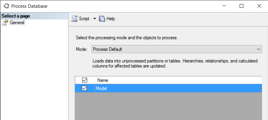
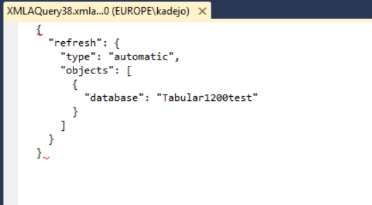
This will generate a JSON-based (TMSL) script instead of an ASSL script:
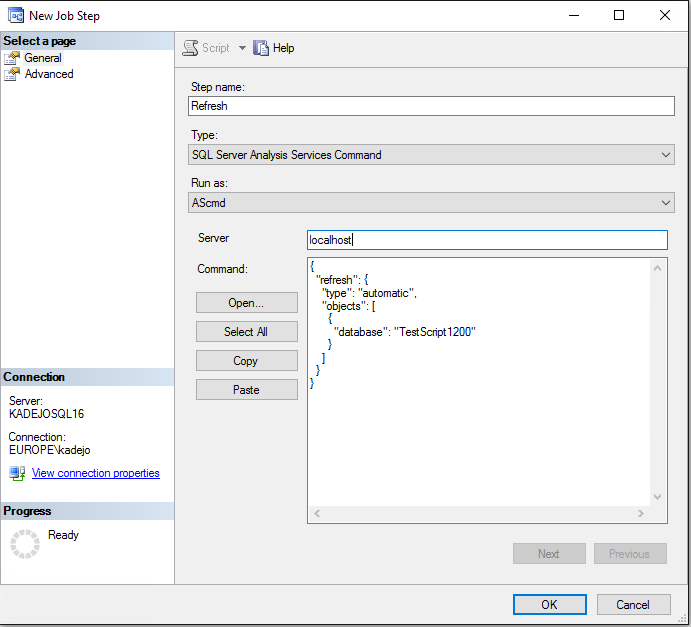
You can now copy in this script to use this in a SQL Server Agent schedule by pasting into the SQL Server Analysis Services Command area:
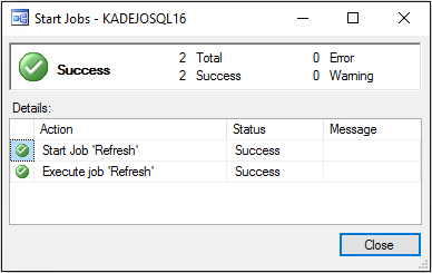
When I run this job, we see that the new TMSL script is executed against the Analysis Services instance:
This implicitly means that Analysis Services now accepts JSON commands as well as ASSL commands on its XMLA endpoints. Any application using XMLA.Execute will be able to send the new TMSL scripts to the CTP3.2 release of Analysis Services against a tabular model created at the 1200 compatibility level.
There are some scenarios that are not yet enabled in this CTP. For the full list, see the release notes. We expect these issues to be resolved in an upcoming CTP. For more details on the TMSL script, see the Tabular Model Scripting Language (TMSL) Reference for XMLA.
Calculated tables
Calculated tables are another CTP 3.2 feature, which allows you to create tables in your model based on a DAX expression. This capability provides you with the flexibility to shape data in any form you want. For example, you can use calculated tables to replicate a table to solve role playing dimensions or to create a new table based on other data in your model. Let’s take a look at two examples using SSDT.
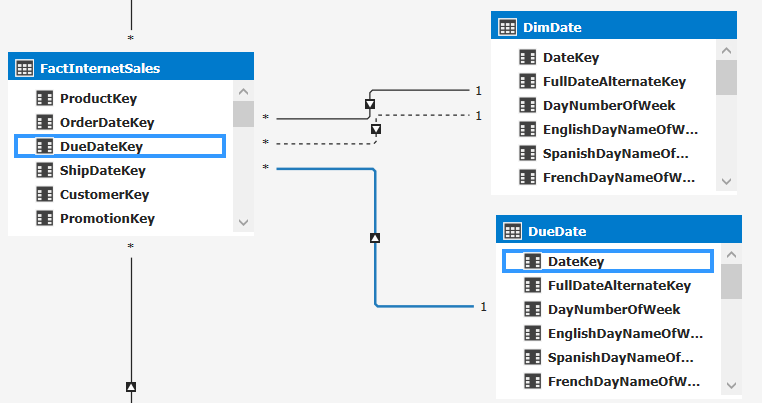
In this model includes two tables, FactInternetSales and DimDate:
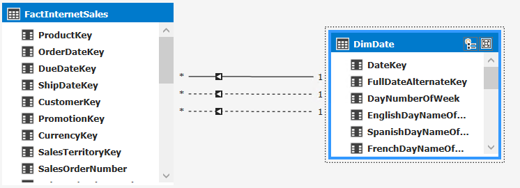
You can see that there are three relationships between FactInternetSales and DimDate: one order date, one for the due date and one for the ship date. It is currently not possible to have all these relationships working at the same time, hence two of the relationship are inactive. However, sometimes you might want your report users to be able to slice by Shipdate instead of Orderdate. One way to accommodate this request is to create a second date table and then create a new relationship to that table. This is easy to do using calculated tables.
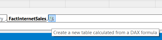
First create a new calculated table by clicking the new calculated table button:
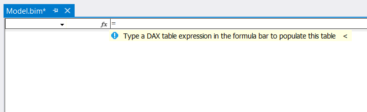
This will add a new empty table where you can add a DAX table expression that allows you to populate the table:
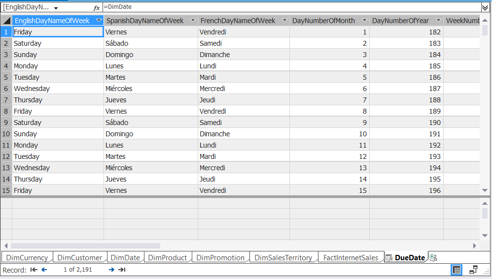
In this case we just want to duplicate the date table so we’ll simply write =DimDate.
This will generate a table exactly like the DimDate table, including any user-defined calculated columns that exist in the table.
You can now create a relationship between the calculated table and the fact table.
Another scenario where calculated tables come in handy is when you need to create a new table based on data in the model using a DAX query. For example, we need to create a table that shows Sales by Color and Currency. This can be accomplished the same way as previously described by creating a new Calculated Table and then adding a DAX formula that summarizes the data:
=SUMMARIZECOLUMNS(DimProduct[Color]
,DimCurrency[CurrencyName]
, "Sales", SUM(FactInternetSales[SalesAmount])
)
This creates a new calculated table that loads the results of the query in memory:
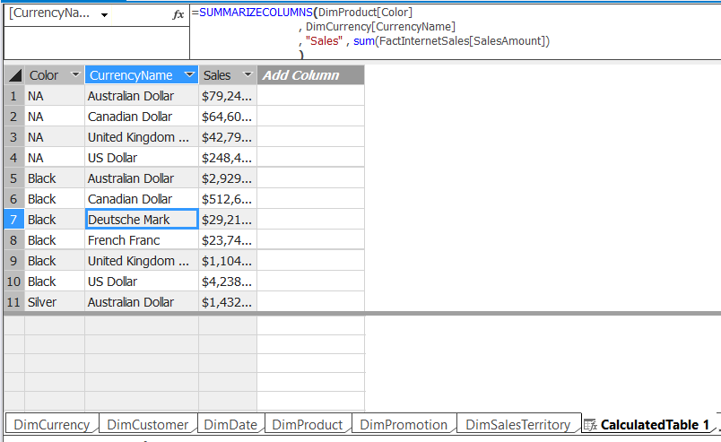
This table can be used exactly the same as if it were imported, very similar to calculated columns.
DirectQuery for models with compatibility level 1200
In CTP3.2 DirectQuery is enabled for models at the 1200 compatibility level. When using DirectQuery in this new compatibility level, you will notice some small differences in how DirectQuery works compared to SQL Server 2014. Let’s walk through the experience of setting up and deploying a DirectQuery model with CTP 3.2.
After creating a Tabular model with compatibility level 1200, we now get the option to turn on DirectQuery mode:
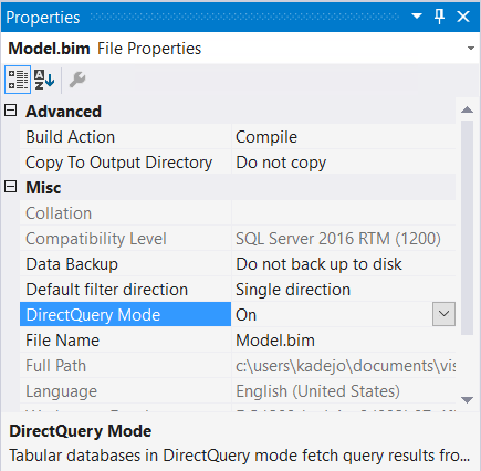
This automatically puts the all the tables and its partitions in the model in “DirectQuery” mode. This will now query the underlying backend data source (SQL Server, Oracle, Teradata, or Analytics Platform) directly instead of using the data loaded into Analysis Services.
Let’s import some data, go through the normal import steps and select several tables from Adventureworks. This is where you will see the first change compared to SQL Server 2014 -- no data is loaded:
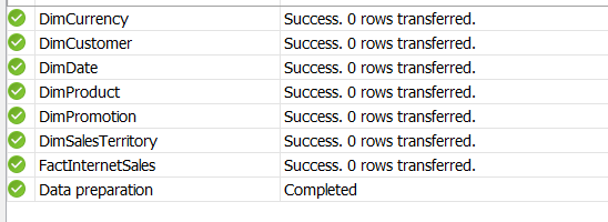
In SQL Server 2014, the model was always automatically set to run in both DirectQuery and in-memory (VertiPaq) mode. This is no longer the case, the model is run in pure DirectQuery mode, with no data loaded in-memory. This of course means that you will not see any data in the data view, but you can still create relationships, measures, and other parts of a model without ever loading data into memory. However, you might want to see at least some data loaded so that you can debug and see what is going on. SSDT already gives you a hint on how to handle this situation:
As you’ve probably gathered, you can create a special partition for every table to be used to create sample views on top of your data. For this simply go to the partition dialog and copy the DirectQuery partition. This will automatically create a new partition that can be used as a sample view on top for your table:
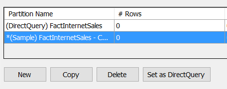
For every DirectQuery partition, you can create as many sample partitions as needed. They will all result in a single sample view of your table. Further on, we’ll take a look on how to use any client app and connect to the sample view of your model instead of the full DirectQuery view.
Now the next thing you might want to do is change the query of the just created sample partition to get a subset of the data. This works just like any other partition as the data in the sample partition is loaded into VertiPaq. This means that you need to process the table:

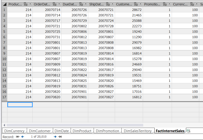
As you can see, this is just a subset of the FactInternetSales table, which contains 60K rows. Once completed, the data will show up in SSDT:
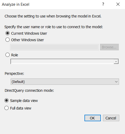
You can also use the same sample view of the data to test your model in Excel by clicking Analyze in Excel:
This will create a new Excel connection that connects to our model with the Sample data view. Behind the scenes, SSDT added an additional item on the connectionstring of the ODC file it generated:
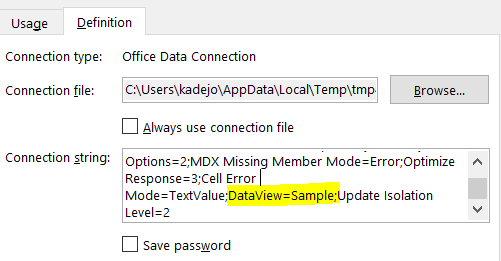
This allows anyone to choose how they want to connect to the model. The Sample data view is currently only available when using DirectQuery.
Now that we’re done modelling we can simply deploy the model to the test server as is. We no longer have to change any settings in the deployment options as was needed in SQL 2014. The model definition now includes the sample partitions, which can be removed later on if no longer needed.
I hope you enjoyed this overview on how DirectQuery works in the new compatibility level, for more information on the full set of new properties please read this help document.
We continue to make updates to DirectQuery in the upcoming months, so stay tuned!
Set the default cross filter direction
In the CTP 3 we released a new relationship type that allows modelers to change the way data is cross filtered between tables. In CTP 3 you could only change this per relationship. In this CTP we now allow you to set the default filter direction for all new relationships being created. On the properties window for the model you can now specify how any new relationships should be created, single or both directions. This will only occur for any new relationships created in this model. If you want to set the default for all projects, you can change the default setting in the Visual Studio options menu under Analysis Services Tabular Designers.
Download now!
To get started, download SQL Server 2016 CTP3.2 here. The corresponding tools, SSDT December 2015 for Visual Studio 2015 can be downloaded here.
Make sure server and tools are the same version to avoid errors related to incompatible components. You might need to uninstall an existing CTP build before getting a newer version.