Creating a Stock Ticker View for Performance Data in PowerPivot

My previous blog post “Analyzing Performance Data in PowerPivot” explained how to create a basic PowerPivot solution to display performance counters for individual servers or server roles in a PivotChart. Subsequently, Jesse Harris, Premier Field Engineer for Microsoft System Center Operations Manager, suggested expanding this solution by providing a view similar to a stock ticker for performance information. Great idea, Jesse! Here is a screenshot of the final solution.

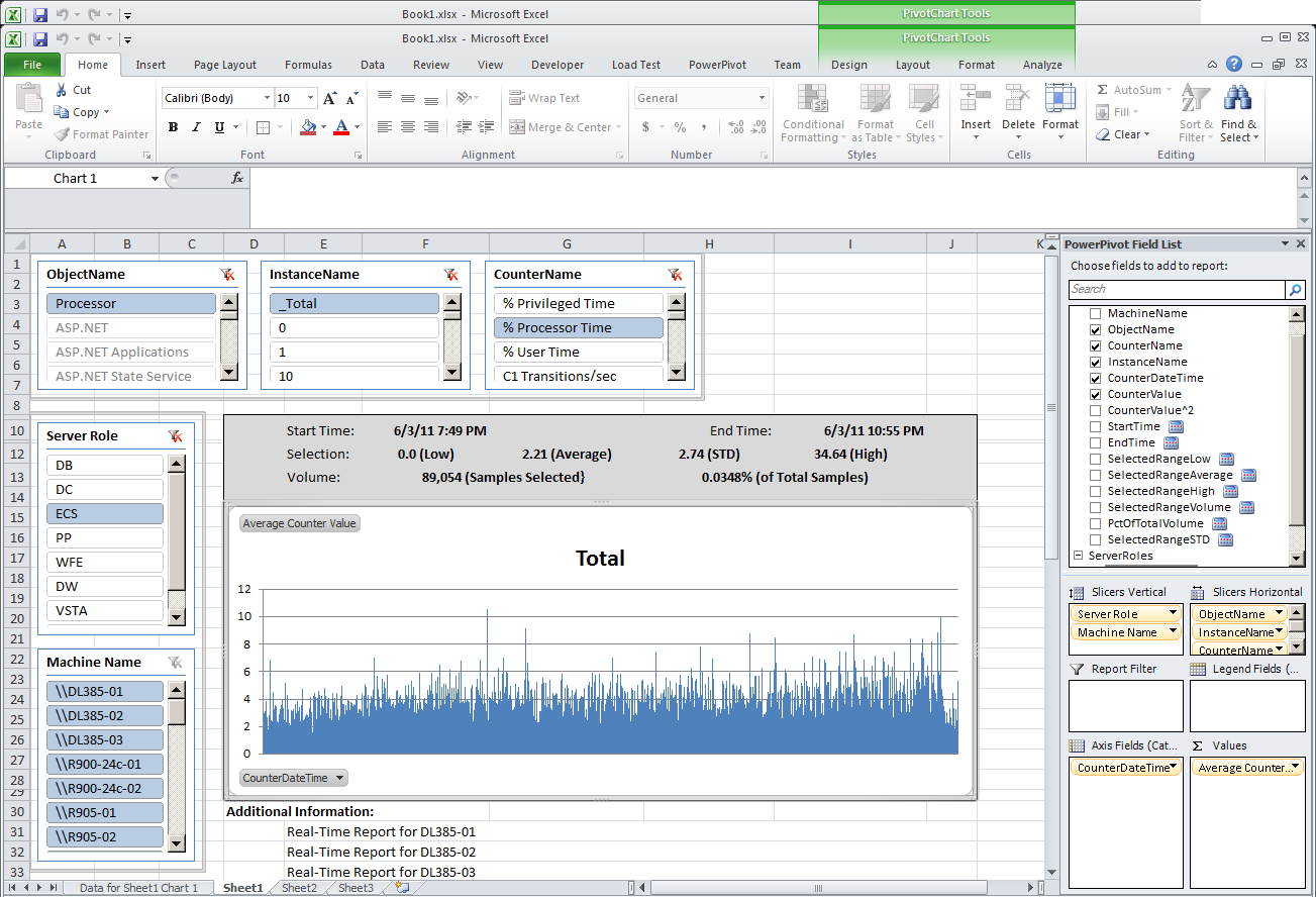
The stock ticker view has three main areas: A header with summary data, the PivotChart, and a section with links to additional information. The PivotChart already exists, which leaves summary header and links to additional information to be implemented. Let’s tackle the summary header first.

The summary header is easily generated by using measures based on straightforward Data Analysis Expressions (DAX). The only exception is the standard deviation (STD) field, which is added separately in a later step. For now, just focus on the simple measures:

1. Start by moving the PivotChart 4 or 5 rows down from its current position on the Excel worksheet to make room for the summary header.
2. Select the cell that previously marked the upper left corner of the PivotChart, such as cell D9, and then on the PowerPivot ribbon, click on the PivotTable button.
3. In the Create PivotTable dialog box, select Existing Worksheet, and then click OK.
4. With the newly created PivotTable selected, on the PowerPivot ribbon, click on the New Measure button.
5. In the Measure Settings dialog box, define the necessary settings according to the following table, and then click OK.

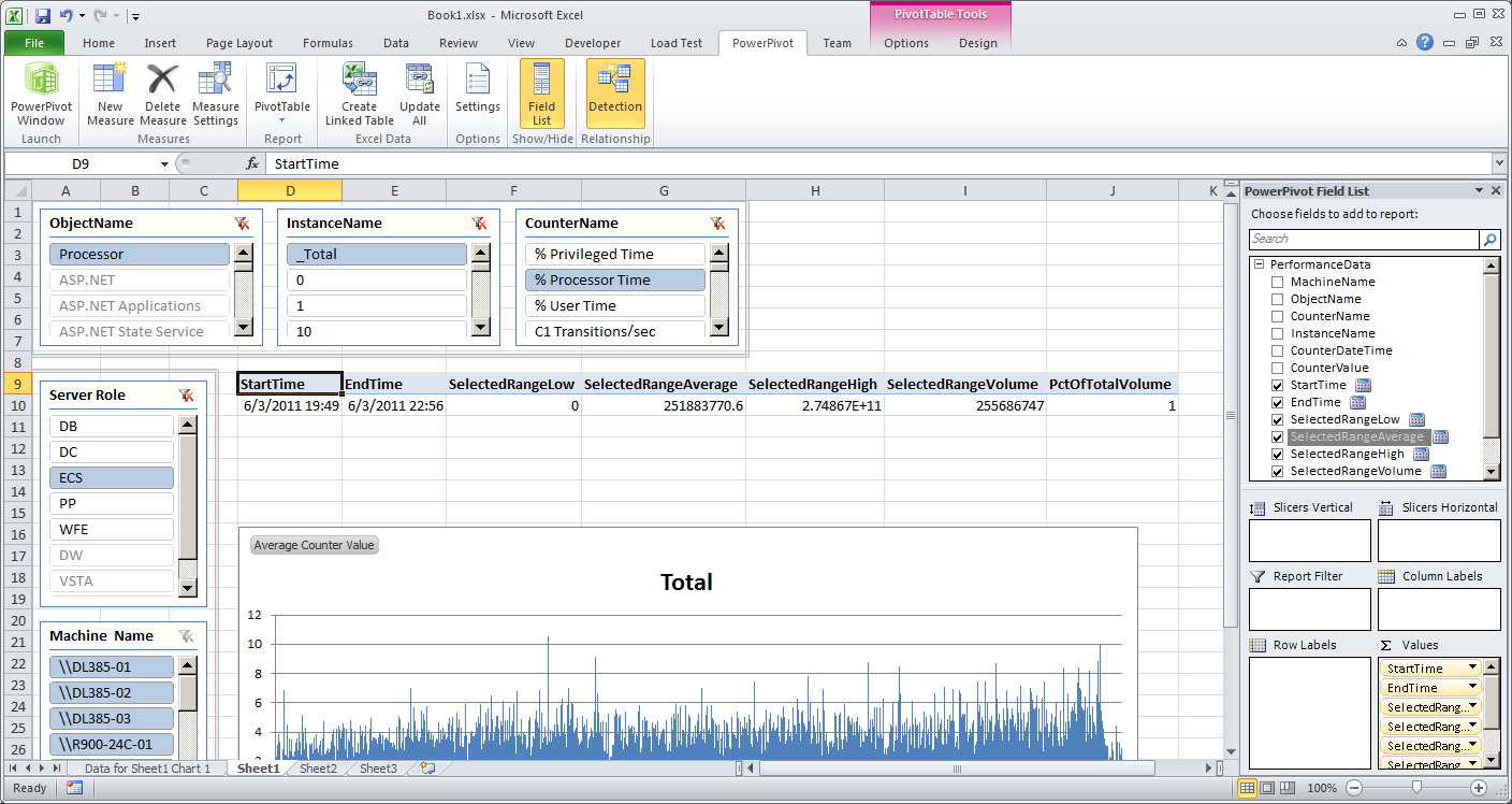
Note that PowerPivot automatically adds the newly created measures as new columns to the selected PivotTable, but the values are most likely incorrect because the PivotTable is not connected to the slicers yet. For example, SelectedRangeVolume does not take the current slicer selection into account and always returns the total number of rows in the PerformanceData table and PctOfTotalVolume is always 1 (see the following screenshot).

To apply the slicers to the PivotTable, follow these steps:

1. With the PivotTable selected, display the Options ribbon in Excel.
2. Under Sort & Filter, click on Insert Slicer, and then select Slicer Connections.
3. In the Slicer Connections (PivotTable1) dialog box, select the checkbox of every listed slicer, and then click OK. Verify that the PivotTable now correctly applies the filter context to the DAX formulas.

Tip: If you like to learn more about measures and filter context, refer to Howie Dickerman’s excellent blog article “DAX (Data Analysis Expressions) Measures in PowerPivot” at https://blogs.msdn.com/b/analysisservices/archive/2010/04/05/dax-data-analysis-expressions-measures-in-powerpivot.aspx.

Now what about the standard deviation? The formula to calculate this value would be SQRT( (SUM(PerformanceData[CounterValue]^2) / COUNTROWS(PerformanceData) ) - ((SUM(PerformanceData[CounterValue]) / COUNTROWS(PerformanceData))^2) ) , but this doesn’t work because the SUM function only accepts a column reference as an argument, yet PerformanceData[CounterValue]^2 isn’t a column (see the following screenshot).

Hence, in order to implement the standard deviation field, you must create a calculated column for PerformanceData[CounterValue]^2:

1. In Excel, switch to the PowerPivot ribbon, and then click on PowerPivot Window.
2. In the PowerPivot window, make sure the PerformanceData table is displayed.
3. Under Add Column, select an empty cell, and then in the formula text box indicated by an fx symbol, type =PerformanceData[CounterValue]^2 and press Enter.
4. Verify that PowerPivot calculates the values for the new column successfully; then right-click the column header named CalculatedColumn1 and select Rename Column.
5. Type CounterValue^2 as the new column name and press Enter.
6. Close the PowerPivot window and save your changes.

At this point, you can repeat the procedure listed earlier in this blog post to create a measure for the standard deviation. Use the following information as a reference.

The measures for the summary header are now complete, yet the PivotTable does not really convey the impression of a stock ticker. In order to rearrange the cells, you must convert the PivotTable into cells with individual formulas:

1. In the Excel worksheet, select the PivotTable.
2. Switch to the Options ribbon, and then under OLAP Tools, select Convert to Formulas. Note that the PivotTable changes to a collection of unformatted cells.
3. Select the first header cell, such as StartTime. Note that the cell uses the CUBEMEMBER function to lookup the cell value in the PowerPivot model, such as =CUBEMEMBER("PowerPivot Data","[Measures].[StartTime]") . Copy the formula without the leading equal sign to the clipboard. Press Escape to exit formula editing mode.
4. Select the first value cell, such as the value for StartTime. Note that the cell uses the CUBEVALUE function to lookup the value in the PowerPivot model, such as =CUBEVALUE("PowerPivot Data",D$9,Slicer_ObjectName,Slicer_InstanceName,Slicer_CounterName,Slicer_Machine_Name,Slicer_Server_Role) . Replace the cell reference in the formula, such as D$9, with the CUBEMEMBER formula you copied to the clipboard in the previous step in order to eliminate the formula’s dependency on another cell’s content.
5. Right-click the value cell, such as the value for StartTime, and select Format Cells. Select an appropriate format, such as Date, 3/14/01 1:30 PM.
6. Repeat the steps for the remaining fields. Use the following table as a reference.

1. Rearrange header and value cells to resemble the header of a stock ticker (see the first screenshot in this blog post) and save your work. Apply formatting, such as boldface and gray cell background, according to your personal preferences.

This concludes the summary header work. Let’s now turn to the links for additional information. These links are an interesting tweak because PowerPivot provides no support for a hyperlink data type out of the box. However, you can construct hyperlinks dynamically by using a hidden PivotTable as an input source for the HYPERLINK function that is available in Excel. Howie Dickerman showed me this tweak. Here are the steps:

1. Switch to Sheet 2, which might already contain the table for machine names and server roles.
2. Select a cell in an empty area, such as cell D1 to the right of the table for the machine names and server roles.
3. On the PowerPivot ribbon, click on the PivotTable button.
4. In the Create PivotTable dialog box, select Existing Worksheet, and then click OK.
5. With the newly created PivotTable selected, in the PowerPivot Field List, expand ServerRoles, and drag the Machine Name node to the Row Labels box. Note that the PivotTable lists all machine names because it isn’t connected to the slicers yet.
6. Display the Options ribbon in Excel, and then under Sort & Filter, click on Insert Slicer, and then select Slicer Connections.
7. In the Slicer Connections (PivotTable2) dialog box, select the checkboxes for the Machine Name and Server Role slicers, and then click OK. Verify that the list of machine names now reflects the selections in the connected slicers.
8. On the Options ribbon, under PivotTable Name, click on Options, and then select Options.
9. In the PivotTable Options dialog box, on the Layout & Format tab, deselect Autofit column widths on update.
10. Switch to the Totals & Filters tab and deselect the checkboxes Show grand totals for rows and Show grand totals for columns. Click OK.
11. Switch to Sheet1, which contains the slicers, summary header, and PivotChart.
12. Select an empty cell underneath the PivotChart, such as cell D30.
13. Type Additional Information: and apply boldface text formatting.
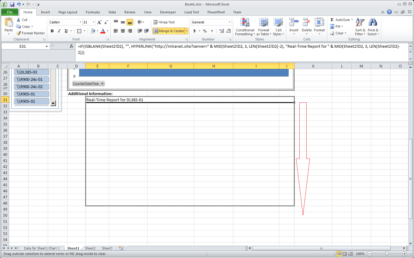
14. Select an empty cell underneath the new Additional Information header, such as E31, and enter the following formula:
    =IF(ISBLANK(Sheet2!D2), "", HYPERLINK("https://intranet.site?server=" & MID(Sheet2!D2, 3, LEN(Sheet2!D2)-2), "Real-Time Report for " & MID(Sheet2!D2, 3, LEN(Sheet2!D2)-2)))
15. Replace the cell reference Sheet2!D2 with the actual cell that contains the first machine name and change the URL part, that is https://intranet.site?server=" & MID(Sheet2!D2, 3, LEN(Sheet2!D2)-2) , as appropriate for your environment. Press Enter.
16. Select the cell with the hyperlink formula as well as the cells to the right for the full width of the PivotChart, such as E31:J31, right-click the selection, and select Format Cells.
17. Switch to the Alignment tab and select the checkbox Merge cells. Click OK.
18. and then drag the outside selection down several rows to extend the series. Fill as many rows as you have servers in the data set. For example, my workbook includes performance data from 30 servers, so I extended the selection down 30 rows. This ensures that every machine name is going to be associated with a hyperlink even if the list of servers in the PivotTable is not filtered by using the Server Role or Machine Name slicers.
19. Verify that the hyperlinks show the correct information and save your work.

The stock ticker view for performance data is now complete. Feel free to add further elements. For example, you could add event log data to the PowerPivot workbook and display relevant information in yet another PivotTable according to the user’s selection in the Server Role and Machine Name slicers. Just make sure you establish appropriate slicer connections as outlined above. In my next blog post, I’m planning to cover PowerPivot storage efficiency. At roughly 250 million rows of performance data, my workbooks tend to be about 800 MB, which might be too large for 32 bit Excel clients. Perhaps something can be done to reduce the workbook size without cutting back on performance analysis. Stay tuned.