Analyzing Event Log Entries in PowerPivot

PowerPivot for Excel is a great analysis tool for information workers. You can import data from any supported data source in your environment or from Azure DataMarket and then analyze that data with supercool Data Analysis Expressions (DAX), but who says PowerPivot is just for information workers? PowerPivot is for everybody! So, why not analyze computer information if you happen to be an IT pro?

If you are an IT pro, you might find it interesting to analyze the Windows Event Log. It’s a great source of valuable information. You might be able to find certain patterns of system errors or security incidents on your servers and workstations. So, let’s load event log data into PowerPivot. One way to accomplish this is to export the data into a CSV file and then import that CSV file into PowerPivot.

Here are the steps:

1. Start Control Panel, and then in Category view, click System and Security, click Administrative Tools, and then double-click Event Viewer.
2. Expand Windows Logs, right-click the desired log, such as System, click Save All Events As, and then in the Save As dialog box, under File Name, type a meaningful name, such as System, and under Save As Type, select CSV (Comma Separated) (*.csv). Click Save.
3. Switch to the PowerPivot window, and then under Get External Data, click on From Text.
4. In the Table Import Wizard that appears, click Browse, and then in the Open dialog box, next to File Name, select Comma Separated Files (*.csv), and select the previously saved file. Click Open.
5. Notice the data preview in the Table Import Wizard. Select the checkbox Use First Row As Column Headers and then click Finish.

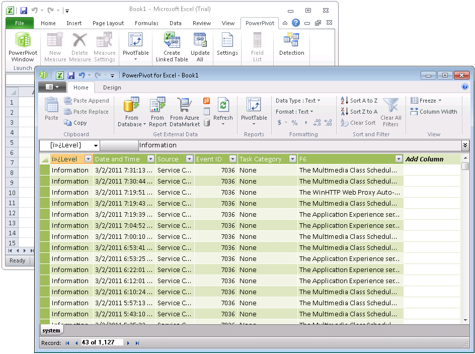
And after removing some invalid characters from the Level heading and renaming the F6 column to Event Details (just right-click the headings and select Rename Column), the data is ready for analysis:

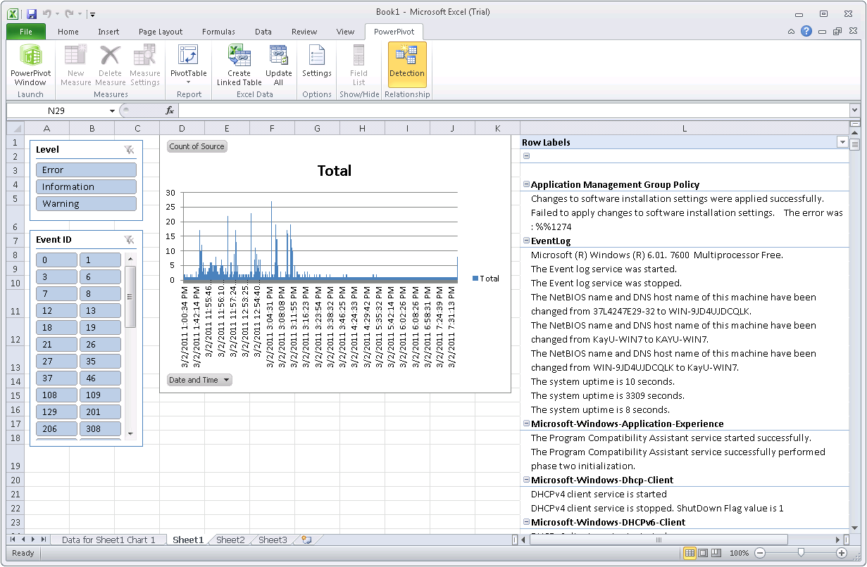
1. Switch to the Excel window, and then on the PowerPivot ribbon, in the Report section, click on the little triangle underneath PivotTable. Select the option Chart and Table (Horizontal).
2. In the Create PivotChart and PivotTable (Horizontal) dialog box, select Existing Worksheet, and then click OK.
3. PowerPivot places an empty chart and an empty PivotTable on the worksheet. Select the chart and then, in the PowerPivot Field List to the right, drag the following fields to the field areas:

1. On the Excel worksheet, click in the area of the PivotTable, and then in the PowerPivot Field List drag the fields Source and Event Details onto the Row Labels field area.
2. On the Excel worksheet, right-click the column that contains the PivotTable, such as column D, and click Column Width. Under Column Width, type 66, and then click OK.
3. Right-click the column that contains the PivotTable again and click PivotTable Options, and then in the PivotTable Options dialog box, clear the checkbox Autofit Column Widths On Update. Click OK.
4. Right-click the column that contains the PivotTable one more time and click Format Cells. Switch to the Alignment tab, and then under Text Control, select the checkbox Wrap Text, and click OK.
5. Test your solution by clicking on a slicer, such as on Information, Error, or Warning. Observe how the data in the chart and in the PivotTable changes, then save your work.

Of course, this is a very basic solution, yet it might nevertheless be useful. Let me know if you find these IT-pro scenarios interesting. In my next blog post, I’m planning to show you how to analyze performance data in PowerPivot. Stay tuned!