Measuring Model Goodness - Part 2

Author: Dr. Ajay Thampi, Lead Data Scientist

Measurability is an important aspect of the Team Data Science Process (TDSP) as it quantifies how good the machine learning model is for the business and helps gain acceptance from the key stakeholders. In part 1 of this series, we defined a template for measuring model goodness specifically looking at classification-type problems. This is summarised in the table below.

In this post, we will look at regression which is another broad class of machine learning problems.

Regression

Regression is the process of estimating a quantitative response. It is a supervised machine learning technique that given a new observation, predicts a real-valued output. This is done based on training data that contains observations whose real-valued outputs are known. In this post, I will look at a specific example of regression which is to predict the dollar value of a home. I will be using the open Boston house prices dataset  which consists of 506 examples, 13 numeric/categoric features such as per capita crime rate, average number of rooms per dwelling, distance to employment centres, etc. and 1 real-valued target representing the median value of a home in 1000s of dollars. More details on the dataset can be found in the Jupyter notebook that I created for this topic on Github.

[caption id="attachment_1005" align="aligncenter" width="500"] Photo by Adrian Scottow on Flickr[/caption]

The business need is to predict the home value (or a real-valued output in the general case) with as low an error as possible and to also be able to see how confident we are of our predictions. These needs can be quantified using the following metrics:

• Error metrics:
  • Mean/Median Absolute Error (MAE)
  • Mean/Median Absolute Percentage Error (MAPE)
  • Root Mean Squared Error (RMSE)
• x% Confidence Interval (CI) or Coefficient of Variation (CoV) for each of our estimates

The 3 metrics that are typically used to quantify the estimation error are MAE, MAPE and RMSE. It is important to understand the differences between them so that the appropriate metric(s) can be used for the problem at hand. Both MAE and RMSE are in the same units of the target variable and are easy to understand in that regard. For the housing price problem, these errors are expressed in dollars and can easily be interpreted. The magnitude of the error, however, cannot be easily understood using these two metrics. For example, an error of $1000 may seem small at first glance but if the actual house price is $2000 then the error is not small in relation to that. This is why MAPE is useful to understand these relative differences as the error is expressed in terms of % error. It is also worth highlighting a difference between MAE and RMSE. RMSE has a tendency to give a higher weight to larger errors - so if larger errors need to be expressed more prominently, RMSE may be the more desirable metric. The M prefix in MAE and MAPE stands for either mean or median and they are both useful in understanding the skew in the error distributions. The mean error would be affected more by outliers than the median.

The CI and CoV metrics can be used to quantify how confident we are in our estimates. By choosing an appropriate threshold for the CoV, we can determine the proportion of cases that we can predict with reasonably high certainty and therefore can potentially automate those. There are of course other ways of quantifying uncertainty [1, 2, 3] but in this post, we will only cover CI and CoV.

We now need to define reasonable baselines to compare our models to.

• Baseline 1: Overall mean (or median)
  • For the housing price example, this is the overall mean value of all houses in Boston.
• Baseline 2: Mean (or median) of a particular group
  • For the housing price example, we can define the group as houses with a certain number of rooms. The predicted value will then be the mean value of the house with those number of rooms. We need to make sure that we have enough samples of data in each of the groups. If there aren't sufficient samples, then we should fall back to the overall mean.
• Baseline 3: Current deployed model
  • Since we do not have access to this model for our example, we will drop this baseline.

The next step is to train a regression model. For this example, I used a pipeline consisting of a standard scaler, PCA to potentially reduce the dimensionality of the feature vector and a gradient boosting regressor to finally predict the value of the house. The quantile loss function was used so that we can predict the median value (alpha = 0.5) and the lower and upper values of the confidence interval (defined by alpha of 0.05 and 0.95 respectively). The code used to build the model can be found here.

Once the models are trained, we then need to evaluate them. We consider the following evaluation metrics:

• Absolute Error (AE): This is defined as | y - ŷ |, where y is the actual value and ŷ is the estimated value
• Absolute Percentage Error (APE): This is defined as | y - ŷ | / y * 100
• Squared Error (SE): This is defined as (y - ŷ)2

We can now translate the above metrics into the final business metrics as follows:

• Mean/Median AE: Mean/median of the absolute errors over all examples in the test set
• Mean/Median APE: Mean/median of the absolute % errors over all examples in the test set
• RMSE: Square root of the mean squared error over all examples in the test set

The above errors are visualised in the figure below.

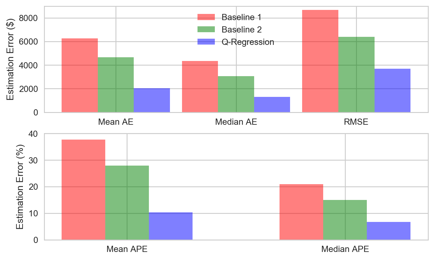
Observations:

• The Quantile Regression (Q-Regression) model does much better than the baselines achieving the lowest values for all error metrics. The mean and median APEs for the model are 10% and 7% respectively.
• The mean and median error metrics show that the distribution of the errors is positively skewed. This is also reflected in the RMSE metric where RMSE is greater than MAE showing the effect of the larger errors.

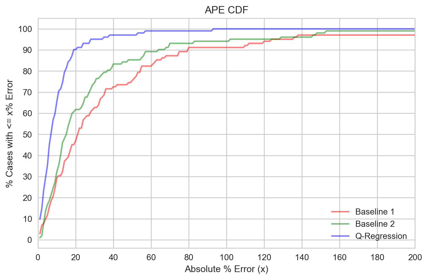
In order to get a better understanding of the distribution of the errors, it is useful to plot the cumulative distribution of the APE. This is shown below.  It can be seen that for the Q-Regression model, 90% of the cases achieve an error of less than 20%. For baselines 1 and 2, we only get roughly 60% and 50% of the cases respectively, with less than 20% error.

Finally, in order to determine which cases we can accurately estimate and in turn automate, we need to look at the confidence interval (CI) and the coefficient of variation (CoV). The 95% CI is estimated using the Q-Regression model by setting the quantile parameter alpha to 0.05 and 0.95. This gives us a rough measure of the spread of the estimate value. We can then compute a rough measure of the CoV by dividing the spread by the median predicted value. We expect to see a higher CoV for an estimate that we are highly uncertain of. Ideally, the CoV will also be correlated with the error metric but that need not always be the case. By setting a threshold on the CoV, we can determine how many cases we can predict with reasonably high certainty and thereby, automate.

In this example, a CoV threshold of 0.625 is chosen. This results in automating roughly 50% of the cases with reasonably high certainty in our estimate value. The figure below shows the box plots of the APE metric for all cases and the 'automatable' cases.

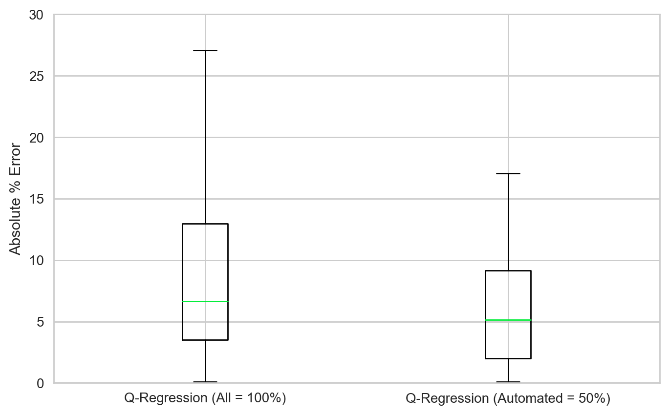
Observations:

• The 50% cases identified as 'automatable' have much lower errors than all the cases.
  • Mean APE drops from 10% to 6%
  • Median APE drops from 7% to 5%
  • Maximum APE drops from 92% to 17%

This concludes the two-part series on measuring model goodness. We've looked at measurability through the lens of the business and defined a template for the entire process for two broad classes of machine learning problems - classification and regression. This is summarised in the table below. For the sake of completeness, the classification column is copied from the table above.

Hope you enjoyed this series. Thanks for reading!