Evaluating Machine Learning models when dealing with imbalanced classes
Sander Timmer, PhD
In real-world Machine Learning scenarios, especially those driven by IoT that are constantly generating data, a common problem is having an imbalanced dataset. This means, we have far more data representing one outcome class than the other. For example, when doing predictive maintenance, there is (far) more data available about the healthy state of a machine than the unhealthy state (given the assumption that machines are not broken all the time). In addition to this, a further complication is that you nearly always care more about predicting the broken, or unhealthy, state correctly (thus the small class) than the normal state (majority class), as this is where the value proposition is. For this reason, evaluation of the model performance, and to understand its business value, takes more than just looking at the overall accuracy. In this blog post I will talk you through a fictive example in which I introduce an additional evaluation metric for machine learning models that can help doing cost-sensitive predictions. Moreover, I will also show how you can easily compare the performance of a single model in various cost settings.
Evaluation metrics in AML today
Many of the normal metrics for evaluating your machine learning model are not that informative for imbalanced classes, with overall accuracy being the worse. To illustrate this, think about a scenario in which on average a machine is failing once every 100 days. Any model that would solely predict healthy state would already by default have an accuracy of 99%!
Luckily, better evaluation metrics are available that will be more effective in determining the overall performance of the model when the classes are imbalanced. Most commonly used metrics, that are by default available in AML, are precision, recall, and F1. Each of these metrics is calculated using the True-Positive (TP), False-Positives (FP), and False-Negatives (FN) rates. To summarize the differences between these metrics, see the following summary:
- Precision denotes the rate of false alarms
- Precision = TP / (TP + FP)
- Recall indicates how many of the failures were detected
- Recall = TP / (TP + FN)
- F1 considers both precision and recall rates and can give a more balanced view.
- F1 = 2 * ((Precision * Recall) / (Precision + Recall))
As these metrics are by default available in AML, they can be used in the model optimization part and the evaluation part.
A less common evaluation metric: Cohen's Kappa coefficient
Another method, that is not available by default, is the Cohen's Kappa coefficient (I will just call this Kappa from now on). The Kappa, by its origin, is capturing the agreement between raters, which can be transformed so it can also work for confusion matrixes. The main reason for me to rely on this metric is that it uses the probability of random agreement. This way it will generate a reliable metric even if the classes are imbalanced. For example, taking the example from the Wikipedia page (Figure 1), it shows that although in both cases the accuracy is 60% (45 + 15 vs 25 + 35) the result is higher for the second case as the by chance agreement is lower in the second.
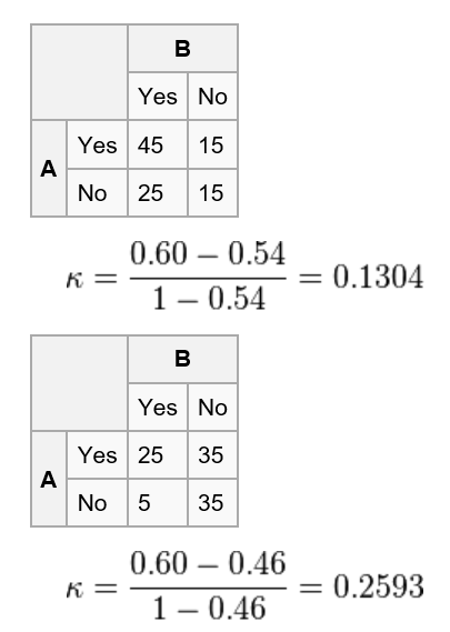
Figure 1 Example results Cohen's Kappa coefficient (https://en.wikipedia.org/wiki/Cohen%27s\_kappa)
Weighted Cohen's Kappa coefficient
Another great value proposition for using Kappa is that you can apply it in a weighted way. In predictive maintenance scenarios often the real business value and costs are different for the various errors you model can make. For example, for each False-Negative (FN) that your model predicts you will have unscheduled failures, which are often both expensive and bad for the perception of your brand. You can often reduce the number of FNs by being more lenient towards predicting the first class, however this will lead to an increase in the number of False-Positives (FP). And each prediction that is FP this will result into unnecessary maintenance, which will have some costs involved to it. Hence, for each business scenario another trade-off will need to be made and by putting weights on the confusion matrix before calculating the Kappa will help you pick the optimal model taking costs into consideration (i.e. cost-sensitive predictions).
The scenario
In this post I will show how I evaluate the results of a binary classification model for predicting if a machine is going to fail in the next 5 days (yes/no are our labels). We have ~100k rows of data that is labelled and scored by a model (score goes from 0 to 1, with 1 being the most likely to fail). To keep things simple, I will not compare different models to each other but showcase within the outcome of the same model I can define an optimal threshold for calling something unhealthy or healthy. In a later state I will also show how I can add weights to my data to model the results of being costs sensitive. All the data and R code to replicate this blog post can be found on my Github repository. I highly recommend you to have a look there as it will also contain an R Markdown script that you can just run to get all the data and visualizations from this post at once.
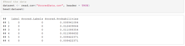
The data
Our dataset looks like as follows. It is a simple data.frame with the 3 columns described above. The names of the columns are like how you get them from an experiment in the Azure Machine Learning studio.
Generating evaluation statistics for our dataset
To get some statistics of how our data looks for each threshold I calculate normal evaluation metrics and Kappa for each threshold from 0 -> 1 with steps of 0.01. This means we have 100 different values to compare and play with.
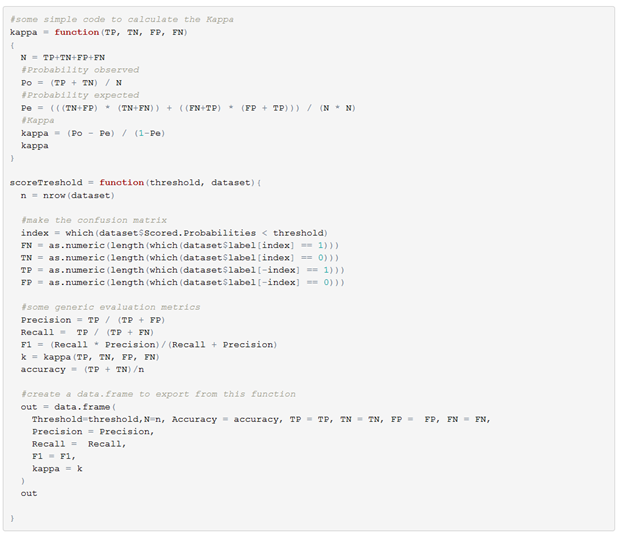
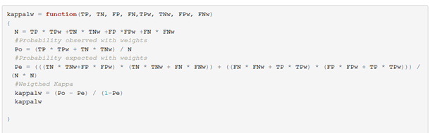
First I defined some code to calculate my statistics and implement a simple way of calculating the Kappa.
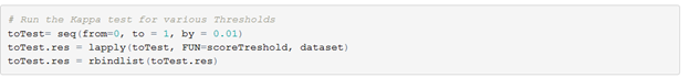
After this I run each threshold that I want to get statistics for through lapply.
Basic evaluation
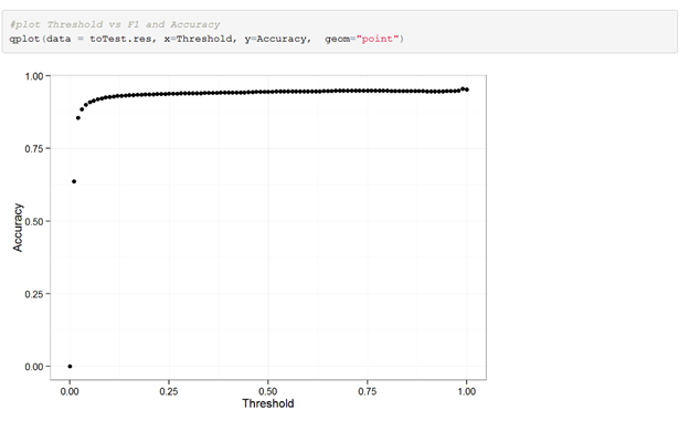
Once again, looking at just accuracy as a metric for evaluation is a bad idea when dealing with such an imbalanced class problem. Nearly for every threshold our model will before great when just looking at this metric.
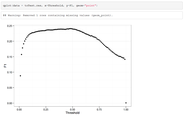
More interesting details about our model can be observed when looking into the F1. When just considering the F1, which is a good way to quickly determine your model performance, it is clear that our model is performing optimal when using 0.47 as a threshold cut-off.
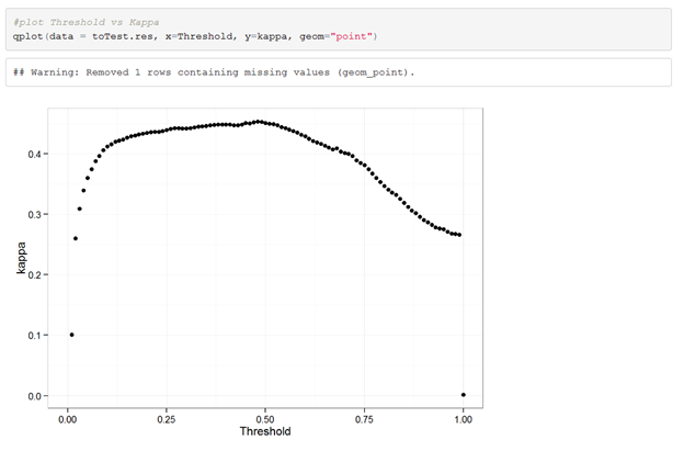
When looking at the Kappa results we instantly see that these results are extremely similar to our F1 results. This is a good thing, as this means we can rely on using F1 metric in Azure Machine Learning studio to optimize our models and define what model should be used for scoring your dataset.
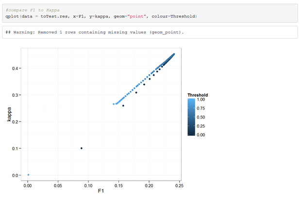
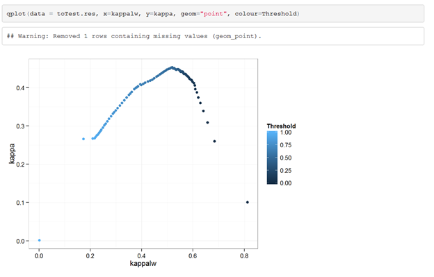
In addition, when we do a direct comparison between Kappa and F1 (colored by Threshold) we observe a very strong correlation between the 2.
Cost sensitive evaluation with weighted Kappa
So, after seeing this you might wonder why we should care about Kappa at all given that F1 does a great job. The main reason for this is that with Kappa we are allowed to introduce some weights to our confusion matrix and start evaluating the true costs that our model might have in the real world.
The code for doing this is very similar to normal Kappa, we just introduce extra variables with the weights for each outcome of the confusion matrix.
If we then run the code for the Thresholds again but now with weights (TP = 1, TN = 1, FP = 0, FN =2) and compare those results to the original Kappa scores we start to see a shift in behaviors. In the given scenario the weighted Kappa actually suggest using a much higher Threshold as it knows that we don't mind having FPs.
Cost sensitive scenarios with weighted Kappa
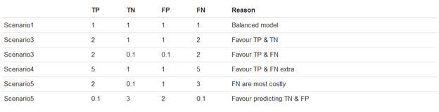
We are now going to compare the weighted Kappa tests for different scenarios. This is to insights into how our current model would perform in different business scenarios. The following 5 scenarios have been constructed:
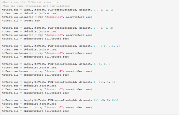
Which we then run through our scripts to calculate all normal evaluation metric, normal Kappa, and the weighted Kappa.
After this step, we have a very long data frame that contains all the information we need to compare the different cost scenarios. We just need to do a tiny reshape trick to make our column in the long format and then we can plot and compare the different cost scenarios.
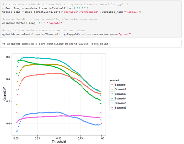
Doing this will help greatly in picking the best performing model for whatever scenario you prefer. As can be seen, there is often agreement that a lower Threshold is better, except when you look at Scenario6, in which we say we are mainly interested in predicting the majority class correct.